Chapter 2 – Simulation Workflows
CST Studio Suite for Particle Dynamics Simulation is designed for ease of use. However, to get started quickly, you need to know a few things. The main purpose of this chapter is to provide an overview of the software’s capabilities. Read this chapter carefully, as this may be the fastest way to learn how to use the software efficiently.
This chapter covers three different workflow examples for Particle Tracking, Particle in Cell (PIC) and Wakefield computations:
1. Workflow Example: Particle Tracking
1.1. Model and simulate a simple electron gun, including a particle simulation (static approximation)
1.2. Parameter studies of the model and automatic optimization of the structure
2. Workflow Example: Electromagnetic Particle in Cell
2.1. Model and simulate a simple output cavity
3. Workflow Example: Wakefield
3.1. Model and simulate a simple pillbox cavity
Simulation Workflow: Particle Tracking
The following example shows, how to set up and run a simple Particle Tracking simulation. Studying this example carefully will allow you to become familiar with many standard operations that are necessary to perform a Particle Tracking simulation within CST Studio Suite. For more information on the physics that can be modelled with the Tracking solver, an overview is provided in Chapter 3 – Solver Overview : Particle Tracking Solver.
Go through the following explanations carefully even if you are not planning to use the software for Particle Tracking simulations. Only a small portion of the example is specific to this particular application type since most of the considerations are general and apply to all solvers and application domains.
At the end of this example, you will find some remarks concerning the differences between the typical simulation procedures for electrostatic and magnetostatic calculations and some useful hints for setting up the Particle Tracking and gun algorithm.
The following explanations always describe the menu-based way to open a particular dialog box or to launch a command. Whenever available, the corresponding toolbar item is displayed next to the command description. Due to the limited space in this manual, the shortest way to activate a particular command (i.e. by pressing a shortcut key or activating the command from the context menu) is omitted. You should regularly open the context menu to check available commands for the currently active mode.
The Structure
Usually an electron gun is only one part of a complex device, for example a particle accelerator. The gun is used to create a collimated particle beam, so that other parts of the device are supplied with a beam of good quality.
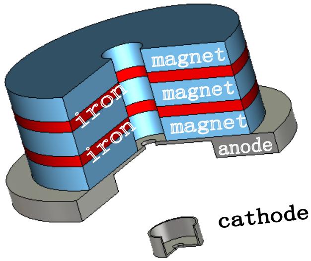
The way this gun works is quite simple. Electrons are emitted from a cathode by a particle source based on space charge limited emission. These particles are accelerated and focused by an anode. Additional focusing is realized by a set of magnets behind the anode.
The following picture shows the structure of interest. It has been sliced open to aid visualization. Anode and cathode consist of perfect electrical conductor (PEC) material whereas the magnetic structure above the anode consists of iron and permanent magnets.
text_image
iron iron magnet magnet magnet anode cathodeBefore you start modeling the structure, let us spend a few moments discussing how to describe this structure efficiently.
In the CST Studio Suite, the user can define the properties of the background material. Anything you do not fill with a particular material will automatically be filled with the background material. For this structure it is sufficient to model anode, cathode, two iron discs and three permanent magnets of the electron gun. The background properties will be set to vacuum.
Your method of describing the structure should therefore be as follows:
- Model cathode and anode of the electron gun.
- Model the two iron discs.
- Model the three permanent magnets.
Create a New Project
After launching the CST Studio Suite, you will enter the start screen showing you a list of recently opened projects and allowing you to select the application that best suits your requirements. The easiest way to get started is to configure a project template, which defines the basic settings that are important for your typical application. Therefore, click on the New Template button in the New Project from Template section within the New and Recent tab.
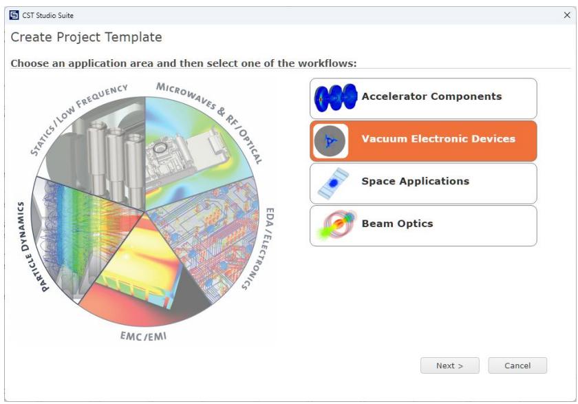
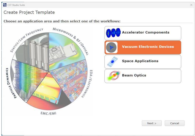
Next, you should choose the application area, Particle Dynamics for the example in this tutorial, and then select the workflow by double-clicking on the corresponding entry.
flowchart
graph LR
  A["Static / Low Frequency"] --> B["Microwaves & RF/OPTICAL"]
  B --> C["EDA/Electronics"]
  C --> D["EMC/EMI"]
  D --> E["Particle Dynamics"]
  E --> F["Static Dynamics"]
For the electron gun, please select Vacuum Electronic Devices Particle Gun Particle Tracking .
Finally, you are requested to select the units that best fit your application. For this example, please select the dimensions as follows:
| Dimensions: | mm |
| Frequency: | Hz |
| Time: | s |
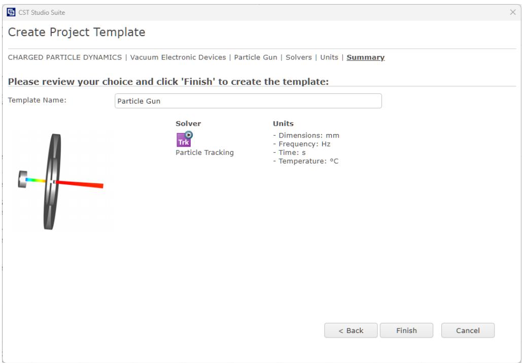
For the specific application in this tutorial the other settings can be left unchanged. After clicking the Next button, you can specify a name for the project template and review a summary of your initial settings:
text_image
CST Studio Suite Create Project Template CHARGED PARTICLE DYNAMICS | Vacuum Electronic Devices | Particle Gun | Solvers | Units | Summary Please review your choice and click 'Finish' to create the template: Template Name: Particle Gun Solver Units Trk Particle Tracking - Dimensions: mm - Frequency: Hz - Time: s - Temperature: °C < Back Finish CancelFinally, click the Finish button to save the project template and to create a new project with the respective settings. CST Studio Suite for Particle Dynamics Simulation will be launched automatically due to the choice of this specific project template within the application area Particle Dynamics.
Please note: When you click again on the File: New and Recent you will see that the recently defined template appears below the Project Templates section. For further projects in the same application area you can simply click on this template entry to launch CST Studio Suite for Particle Dynamics Simulation with useful basic settings. It is not necessary to define a new template each time. You are now able to start the software with reasonable initial settings quickly with just one click on the corresponding template.
Please note: All settings made for a project template can be modified later during the construction of your model. For example, the units can be modified in the units dialog box (Home: Settings Units ) and the solver type can be selected via the Home: Simulation Setup Solver drop-down list.
Open the Tracking QuickStart Guide
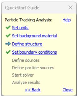
An interesting feature of the online help system is the QuickStart Guide, an electronic assistant that will guide you through your simulation. If it does not show up automatically, you can open this assistant by selecting QuickStart Guide from the dropdown list next to the Help button in the upper right corner.
The following dialog box should then be visible at the upper right corner of the main view:
text_image
QuickStart Guide Particle Tracking Analysis: Help ✓ Set units ✓ Set background material ▶ Define structure ✓ Set boundary conditions Define sources Define particle sources Start solver Analyze results << Back CloseAs the project template has already set the solver type, units, background material and boundary conditions, the Particle Tracking Analysis is preselected and some entries are marked as done. The blue arrow always indicates the next step necessary for your problem definition. You do not have to follow the steps in this order, but we recommend to follow this guide at the beginning to ensure that all necessary steps have been completed.
Look at the dialog box as you follow the various steps in this example. You may close the assistant at any time. Even if you re-open the window later, it will always indicate the next required step.
If you are unsure of how to access a certain operation, click on the corresponding line. The QuickStart Guide will then either run an animation showing the location of the related menu entry or open the corresponding help page.
Define the Units
The Particle Gun template has already applied some settings for you. The defaults for this structure type are geometrical units in mm and time in s. You can change these settings in the units dialog box (Home: Settings Units ), but for this example you should just leave the settings as specified by the template. Additionally, the used units are also displayed in the status bar:

Define the Background Material
As discussed above, the structure will be described within vacuum. The material type Normal is set as default background material in the Particle Gun template. For this example, you do not need to make any changes as the default properties of the material type Normal are those of vacuum. In case you need to change the properties, you may do so in the corresponding dialog box Simulation: Settings Background
Model the Structure
The basic settings have been made, now we are able to set up the structure. Since the electron gun is rotationally symmetric, a special but very efficient technique can be used to design the structure. First, the cathode is created.
- Open the Rotate Profile dialog box Modeling: Shapes Rotate Face to create the cathode.
- Press the ESC key to show the dialog box. Do not click a point in the working plane.
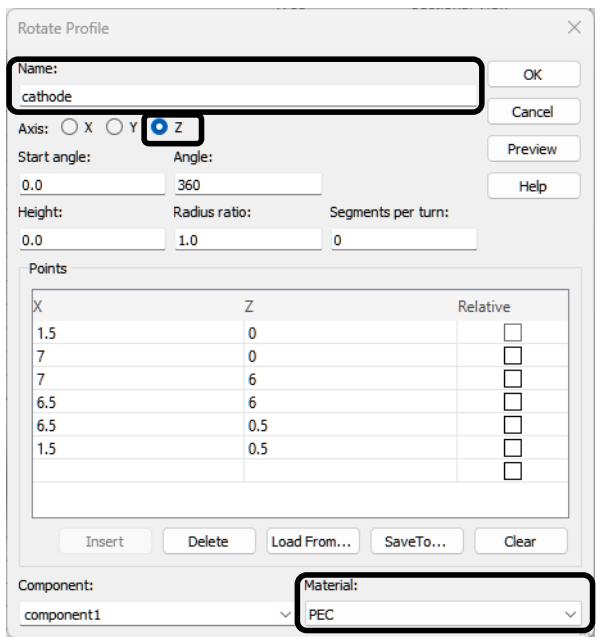
text_image
Rotate Profile Name: cathode Axis: ○ X ○ Y ● Z Start angle: Angle: 0.0 360 Height: Radius ratio: Segments per turn: 0.0 1.0 0 Points X Z Relative 1.5 0 7 0 7 6 6.5 6 6.5 0.5 1.5 0.5 Insert Delete Load From... SaveTo... Clear Component: component1 Material: PEC- Enter the name "cathode" and choose Z as axis of rotation. Set the material to PEC. Now enter the polygon data as shown in the table below.
| x | z |
| 1.5 | 0.0 |
| 7.0 | 0.0 |
| 7.0 | 6.0 |
| 6.5 | 6.0 |
| 6.5 | 0.5 |
| 1.5 | 0.5 |
- You may click the Preview button during the construction to get a preview of the solid. This makes it easy to detect any possible mistakes when entering the data.
The dialog box should now look like in the picture above. Click the OK button to confirm your settings and to construct the cathode.
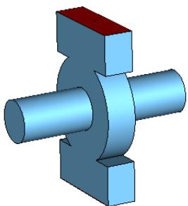
- The structure is displayed in the working plane and now your cathode should look like this:
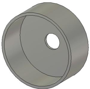
natural_image
3D rendered image of a cylindrical mechanical part with a central hole (no text or symbols)One part of the cathode is still missing, the inner cylinder. We will need this inner cylinder to define the particle source. To create this cylinder, open the Cylinder dialog Modeling: Shapes Cylinder . Press the ESC key to show the dialog box.
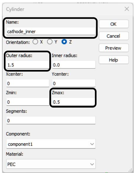
text_image
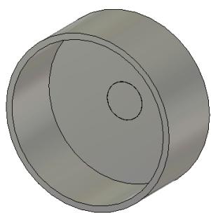
Cylinder Name: cathode_inner Orientation: X Y Z Outer radius: 1.5 Inner radius: 0.0 Xcenter: Ycenter: 0 0 Zmin: Zmax: 0 0.5 Segments: 0 Component: component1 Material: PECChange the name the name to "cathode_inner", enter an Outer radius of 1.5 and Zmax of 0.5. Click the OK button to confirm your changes. The cylinder should fit perfectly into the hole of the solid cathode:
natural_image
3D rendered diagram of a cylindrical object with a circular cutout and center hole (no text or symbols)- The construction of the cathode is completely finished and now we will construct the anode in the same way as we constructed the outer cathode. Open the Rotate Profile dialog box Modeling: Shapes Rotate Face .
-
Press the ESC key to show the dialog box. Do not click a point in the working plane.
-
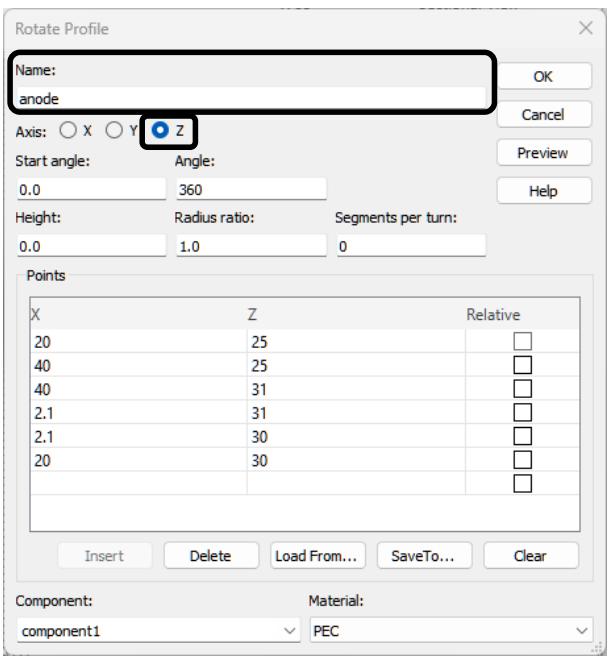
Enter the name "anode" and choose z as axis of rotation. The material PEC should be automatically selected.
text_image
Rotate Profile Name: anode Axis: X Y Z Start angle: Angle: 0.0 360 Height: Radius ratio: Segments per turn: 0.0 1.0 0 Points X Z Relative 20 25 40 25 40 31 2.1 31 2.1 30 20 30 Insert Delete Load From... SaveTo... Clear Component: Material: component1 PECNow enter the polygon data as shown in the following table:
| x | z |
| 20.0 | 25.0 |
| 40.0 | 25.0 |
| 40.0 | 31.0 |
| 2.1 | 31.0 |
| 2.1 | 30.0 |
| 20.0 | 30.0 |
Your dialog box should now look like in the picture above. Click the OK button to confirm your changes. The creation of the anode is complete and the whole structure should look like this (rotated for better visibility):
natural_image
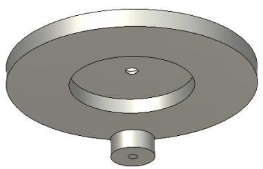
3D rendered mechanical part with concentric circular features and a central hole (no text or symbols)- As you might have noticed, the magnetic part of the structure is still missing. First, we will construct the three vacuum discs that will serve as permanent magnets. To create one disc, open the Cylinder dialog box Modeling: Shapes Cylinder . Press the ESC key to show the dialog box.
- Enter the name "magnet", outer radius 32.8 and the inner radius 5.8. The z range extends from 31 to 37.9 mm. Change the material to vacuum. Click the OK button to confirm your changes.
text_image
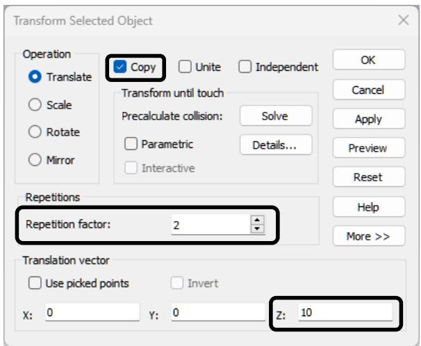
Cylinder Name: magnet Orientation: X Y Z Outer radius: Inner radius: 32.8 5.8 Xcenter: Ycenter: 0 0 Zmin: Zmax: 31 37.9 Segments: 0 Component: component1 Material: Vacuum- Since the same cylinder exists three times, we will use the transform dialog box to create the missing two cylinders. First, select the solid "magnet" in the navigation tree NT: Components \(\Rightarrow\) component 1 magnet.
- Open the Transform Selected Object dialog box Modeling: \(T o o I s \hookrightarrow T r a n s f o r m \tilde { \mathbf { a } } ^ { \perp }\) to copy the cylinder.
text_image
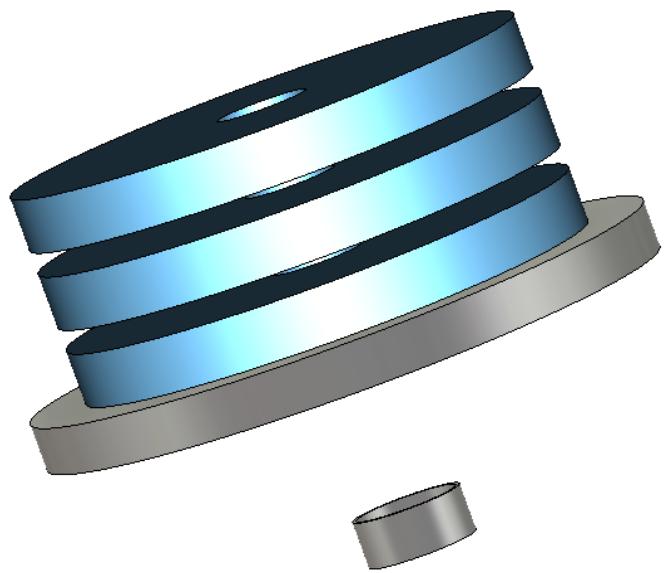
Transform Selected Object Operation Translate Scale Rotate Mirror Copy Unite Independent OK Cancel Apply Preview Reset Repetitions Repetition factor: 2 More >> Translation vector Use picked points Invert X: 0 Y: 0 Z: 10Enable the checkbox Copy. Then enter a translation of 10 in z-direction. Change the Repetition factor to 2 and click the OK button to confirm your changes. The structure should now look like this:
natural_image
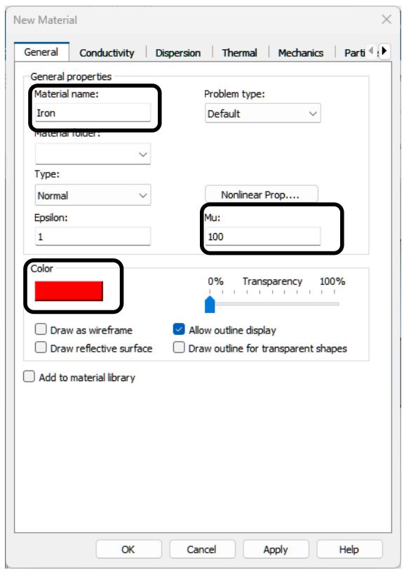
3D rendered mechanical component with layered blue and gray sections, no visible text or symbols- Before the iron discs will be defined, we create a new and simple iron material. To do this, open the material dialog box Modeling: Materials New/Edit New Material. Change the Material name to "Iron", the Color to red and value of Mu to 100 like in the picture below. Now we have quickly defined a simple iron material. Click the OK button to confirm your changes and to leave this dialog box.
text_image
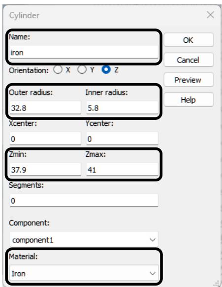
New Material General Conductivity Dispersion Thermal Mechanics Parti General properties Material name: Iron Problem type: Default Material folder: Type: Normal Epsilon: 1 Nonlinear Prop.... Mu: 100 Color 0% Transparency 100% Draw as wireframe Allow outline display Draw reflective surface Draw outline for transparent shapes Add to material library OK Cancel Apply Help- The iron discs are created in the same way as the magnets. Open the cylinder dialog Modeling: Shapes Cylinder . Press the ESC key to show the dialog box.
text_image
Cylinder Name: iron Orientation: X Y Z Outer radius: Inner radius: 32.8 5.8 Xcenter: Ycenter: 0 0 Zmin: Zmax: 37.9 41 Segments: 0 Component: component1 Material: Iron- Enter the Name "iron", an Outer radius of 32.8 and Inner radius of 5.8. The z range extends from 37.9 to 41 mm. Change the material to the new material \(" \ln 0 \mathsf { n } " .\) . Your dialog box should now look like the above picture.
- Finally click the OK button and confirm your changes. To create the second iron disc, we will use the transform mechanism again. Select the solid \(" \mathsf { i r o n " }\) in the navigation tree.
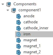
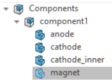
flowchart
graph TD
  A["Components"] --> B["component1"]
  B --> C["anode"]
  C --> D["cathode"]
  D --> E["cathode_inner"]
  E --> F["iron"]
  F --> G["magnet"]
  G --> H["magnet_1"]
H --> I["magnet_2"]- Open the Transform Selected Object dialog box Modeling: Tools Transform \(\hat { \mathbf { a } } ^ { \tt a }\) to copy the cylinder.
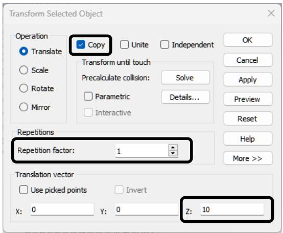
text_image
Transform Selected Object Operation Translate Scale Rotate Mirror Copy Unite Independent OK Cancel Apply Preview Reset Repetitions Repetition factor: 1 Translation vector Use picked points Invert X: 0 Y: 0 Z: 10- Select Copy and enter a translation of 10 in z-direction. Click the OK button to confirm your changes. Now the structure should look like this:
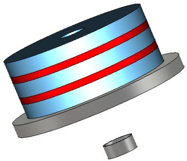
natural_image
3D rendered mechanical component with layered structure and two small cylindrical parts (no text or symbols)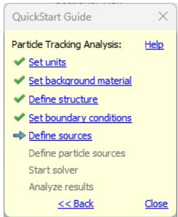
text_image
QuickStart Guide Particle Tracking Analysis: Help ✓ Set units ✓ Set background material ✓ Define structure ✓ Set boundary conditions ▶ Define sources Define particle sources Start solver Analyze results << Back Close- The structure creation part is finished and we can start to define the sources, i.e. potentials, magnets and particle sources.
Congratulations! You have just created your first Particle Tracking structure within CST Studio Suite.
Define Potentials and Magnets
With all components for the electrostatic part of the configuration defined, the appropriate potentials can be set. First, define the potentials of the cathode and anode:
- Select Simulation: Sources and Loads Static Sources Electric Potential and double-click on the surface of the “cathode” solid in the working plane. Press the Return key to finish your selection and to open the Define Potential dialog box.
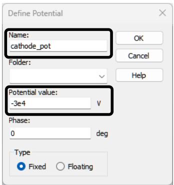
text_image
Define Potential Name: cathode_pot Folder: Potential value: -3e4 V Phase: 0 deg Type Fixed Floating- Enter the name "cathode_pot" and a value of -3e4 V. As usual, click the OK button to confirm your changes.
- In the same way, the potential for the anode is defined. Select Simulation: Sources and Loads Static Sources Electric Potential and double-click on the surface of the anode. Press the Return key to finish your selection and to open the Define Potential dialog box.
- Enter the name "anode_pot" and a value of 0 V. Click the OK button to confirm your changes.
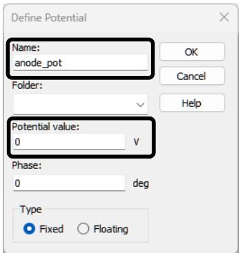
text_image
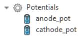
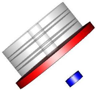
Define Potential Name: anode_pot Folder: Potential value: 0 V Phase: 0 deg Type Fixed Floating- If you now select the potential folder in the navigation tree your structure should look like the picture below:
natural_image
3D rendering of a metallic panel with red and blue side indicators (no text or symbols)Note: As the solids "cathode" and "cathode_inner" are in direct contact, both have the same potential. That means "cathode_inner" also has a potential of -30 kV.
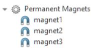
- After the potential definition is finished, we will create three permanent magnets for the three vacuum discs. To define the first magnet select Simulation: Sources and Loads Static Sources Permanent Magnet .
- Then select the solid that should become a permanent magnet. Thus, double-click on the vacuum disc named "magnet".
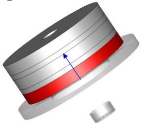
natural_image
3D rendered mechanical component with red and gray bands and a blue directional arrow (no text or symbols)- The Define Magnet dialog box opens. Ensure that the vector components are set to X: 0, Y: 0, Z: 1 and Inverse direction is not checked. Enter a value of 0.02 T for the remanent flux. Leave the other settings unchanged and click OK to confirm.
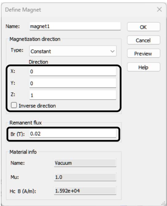
text_image
Define Magnet Name: magnet1 Magnetization direction Type: Constant Direction X: 0 Y: 0 Z: 1 □ Inverse direction Remanent flux Br (T): 0.02 Material info Name: Vacuum Mu: 1.0 Hc B (A/m): 1.592e+04- In the same way, define magnets for the vacuum solids "magnet_1" and "magnet_2" in z-direction. The solid "magnet_1" should be the vacuum disc in the middle of the three discs.
| solid | name | X | Y | Z | Inverse direction | Br (T) |
| magnet | magnet1 | 0 | 0 | 1 | $\square$ | 0.02 |
| magnet_1 | magnet2 | 0 | 0 | 1 | $\checkmark$ | 0.01 |
| magnet_2 | magnet3 | 0 | 0 | 1 | $\square$ | 0.01 |
- If you now select the Permanent Magnets folder in the navigation tree you should see the following picture:
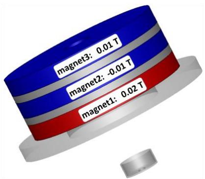
text_image
magnet3: 0.01 T magnet2: -0.01 T magnet1: 0.02 T- Potential and magnet definitions are now complete.
In practice, it is advisable to visualize and refine the mesh before the particle source is defined. The reason is that the number of emission points of the particle source can depend on the mesh settings. This matter is discussed in detail in the later chapter Define Particle Sources.
Visualize and Refine the Mesh
By default, the Particle Tracking solver uses a hexahedral mesh for computing electrostatic and magnetostatic fields. This is the optimal choice for axis-aligned structures as used in this example. However, especially when surfaces in the vicinity of the particle trajectories are curved, their representation by tetrahedral mesh cells might be better-suited and will deliver more accurate results. In order to keep the focus on the simulation workflow itself, we will deal with tetrahedral meshes in a later, more specialized section.
The mesh generation for the structure’s analysis is performed automatically based on an expert system. However, in some situations it may be helpful to inspect the mesh to improve the simulation speed by changing the parameters for the mesh generation.
The mesh can be visualized by entering the mesh view Home: Mesh Mesh View . For this structure, the mesh information will be displayed as follows:
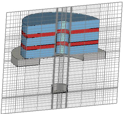
natural_image
3D CAD model of a cylindrical mechanical component with red and blue bands, enclosed within a wireframe grid (no text or symbols)One 2D mesh plane is visible at a time. You can modify the orientation of the mesh plane by adjusting the selection in the Mesh: Sectional View Normal dropdown list or just by pressing the X/Y/Z keys. Move the plane along its normal direction using the Up/Down cursor keys. The current position of the plane will be shown in the Mesh: Sectional View Position field.
There are some thick mesh lines shown in the mesh view. These mesh lines represent important planes (so-called snapping planes) at which placement of mesh lines is considered necessary by the expert system. You can control these so-called snapping planes in the Special Mesh Properties dialog by selecting Simulation: Mesh Global Properties Specials Snapping.
In many cases, the automatic mesh generation will produce a reasonable initial mesh, but in our case, we will refine the mesh in the cathode region to have a finer mesh resolution for the particle beam.
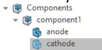
- Make sure you are in the mesh view mode. Select the solid cathode in the navigation tree NT: Components component1 cathode.
- Open the dialog box Mesh: Mesh Control Local Properties to modify the local mesh settings of the cathode. In the General tab, choose Absolute value from the Volume refinement drop-down list. This brings up the Use same setting in all three directions checkbox. Uncheck that box and change the step width in x and y to a value of 0.4.
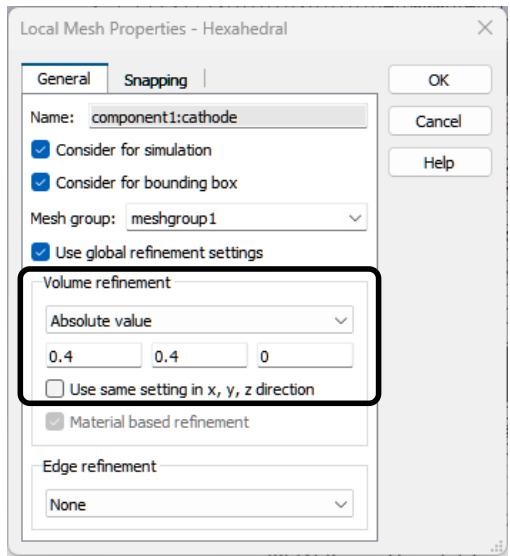
text_image
Local Mesh Properties - Hexahedral General Snapping Name: component1:cathode ✓ Consider for simulation ✓ Consider for bounding box Mesh group: meshgroup1 ✓ Use global refinement settings Volume refinement Absolute value 0.4 0.4 0 □ Use same setting in x, y, z direction ✓ Material based refinement Edge refinement None OK Cancel Help- Confirm your changes as usual by clicking on the OK button. The dialog box closes and you can see the modified mesh.
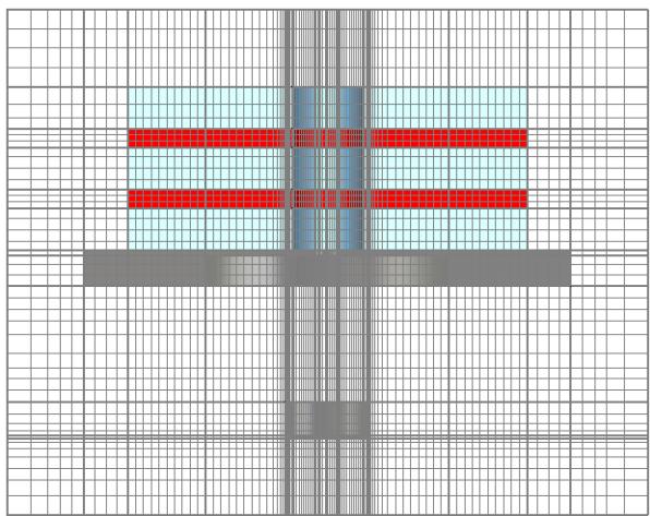
natural_image
Abstract geometric pattern with red horizontal stripes on a grid background (no text or symbols)The number of mesh cells should be 497,536. You can get this information from the status bar.

You can now leave the mesh inspection mode via Mesh: Close Close Mesh View .
Define Particle Sources
A particle source is a shaped surface of a component where charged particles enter the computational domain under a specific emission condition, which is determined by the emission model settings. Such a source is often located on the surface of a PEC solid, but it can also be defined on the surface of any arbitrary material. In our case the particle source will be placed on the inner cathode. To facilitate the selection of the surface of the inner cathode, some solids will be hidden.
- Select "cathode" and "cathode_inner" in the navigation tree. Use the Shift key for multi-selection. Select the option View: Visibility Hide Hide Unselected. Now we are able to define the particle source.
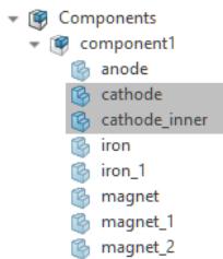
flowchart
graph TD
  A["Components"] --> B["component1"]
  B --> C["anode"]
  C --> D["cathode"]
  D --> E["cathode_inner"]
  E --> F["iron"]
  F --> G["iron_1"]
  G --> H["magnet"]
  H --> I["magnet_1"]
I --> J["magnet_2"]- Select Simulation: Sources and Loads Particle Sources Particle Area Source and select the inner surface of the solid "cathode_inner" by doubleclicking it. Make sure that the surface is highlighted when you move the mouse cursor away from the surface.
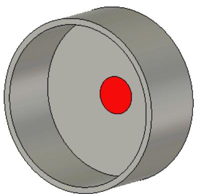
natural_image
3D rendered diagram of a cylindrical object with a red center and concentric rings (no text or symbols)- After selecting the emission surface, press the Return key to open the Define Particle Area Source dialog box. Here, the particle type and particle density at the previously selected surface are adjustable. Change the Tracking emission model to Space charge. The blue points in the preview visualize the particle emission points. Their density can be influenced using the Number of emission points slider. An increase of the number of emission points leads to a smoother current density. The checkbox Adjust density to mesh should be enabled if the emission model Space charge is chosen. Otherwise, the number of emission points might be too low to obtain good simulation results and then has to be increased manually when refining the mesh.
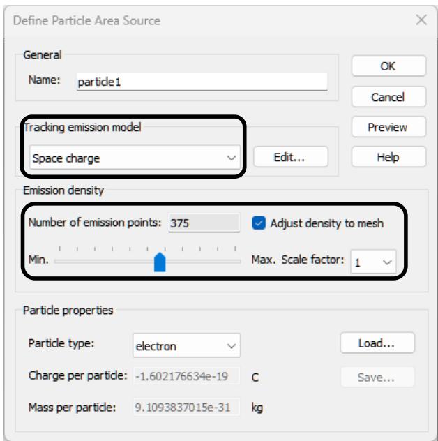
text_image
Define Particle Area Source General Name: particle1 Tracking emission model Space charge Edit... Help Emission density Number of emission points: 375 Adjust density to mesh Min. Max. Scale factor: 1 Particle properties Particle type: electron Load... Charge per particle: -1.602176634e-19 C Save... Mass per particle: 9.1093837015e-31 kgNote: As seen in the lower part of the dialog box, standard or user-defined particle types can be specified. A particle definition library allows you to export such user-defined particle definitions to a database and also to import them. This library is accessible through the Load and Save buttons. In this example, we keep the default particle type electron.
- Move the Number of emission points slider until the number is 375. For finecontrol, you can use the left/right arrow keys while the slider is focused. To change the emission model settings, click the Edit button next to the emission model drop down list. The SCL Emission Settings dialog box opens:
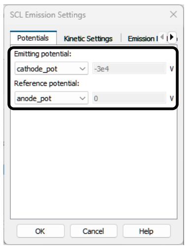
text_image
SCL Emission Settings Potentials Kinetic Settings Emission I Emitting potential: cathode_pot -3e4 V Reference potential: anode_pot 0 V OK Cancel Help- An emission model describes the conditions particles need to fulfill in order to be emitted into free space. For instance, the space charge emission model allows particles to be emitted as long as an electric field perpendicular to the emitting surface is present. If not already preselected, make the following adjustments inside the dialog box on the Potentials tab: Change the emitting potential to "cathode_pot" and the reference potential to "anode_pot". Click the OK button to confirm your changes. The particle source should now look like this:
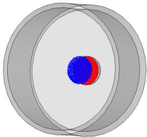
natural_image
Diagram showing concentric circular shapes with a central blue and red dot, no text or symbols presentNote:
The red triangular mesh shows the discretization of the cathode surface, while the blue points visualize the start positions of the particles for the simulation. In this case, the emission model Space charge requires the start positions to be shifted a little bit away from the cathode surface. This shifting is done automatically depending on the mesh close to the cathode.
- We have finished the particle source definition and can now leave the Define Particle Area Source dialog box by clicking the OK button again.
- Since some solids are currently hidden, we have to unhide them to see the whole structure again. Select View: Visibility Show (dropdown list) Show All. It is often helpful to hide some solids in order to select faces inside a structure.
The particle source is now defined and ready for emission. Before you continue, have a look at the QuickStart Guide to see the next steps.
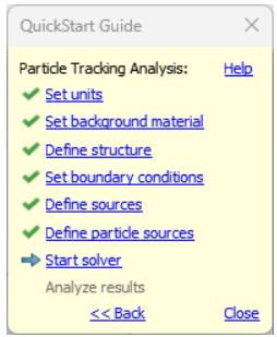
text_image
QuickStart Guide Particle Tracking Analysis: Help ✓ Set units ✓ Set background material ✓ Define structure ✓ Set boundary conditions ✓ Define sources ✓ Define particle sources → Start solver Analyze results << Back CloseThe point “Set boundary conditions” has already been set to finished as the boundaries were defined by the Particle Gun template. Nevertheless, the boundary conditions will be discussed in the next section to illustrate the basics of the boundary condition setup.
Define Boundary Conditions
The simulation will be performed only within the bounding box of the structure, the socalled computational domain. You can specify certain boundary conditions for each plane (Xmin, Xmax, Ymin, Ymax, Zmin, Zmax) of the computational domain. These boundary conditions reflect the appropriate behavior of the surrounding world.
The boundary conditions are specified in a dialog box which can be opened by choosing Simulation: Settings Boundaries .
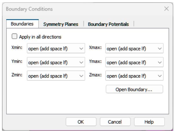
text_image
Boundary Conditions Boundaries Symmetry Planes Boundary Potentials Apply in all directions Xmin: open (add space If) ✓ Xmax: open (add space If) ✓ Ymin: open (add space If) ✓ Ymax: open (add space If) ✓ Zmin: open (add space If) ✓ Zmax: open (add space If) ✓ Open Boundary... OK Cancel HelpWhile the boundary dialog box is open, the boundary conditions are visualized in the structure view as shown in the next picture.
You can change boundary conditions from within the dialog box or interactively in the view. Select a boundary by double-clicking on the boundary symbol within the view and select the appropriate type from the context menu.
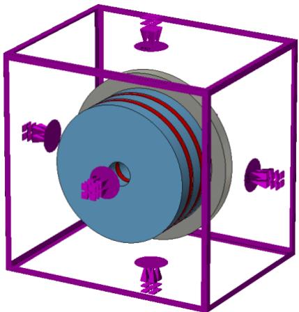
natural_image
3D rendering of a cylindrical mechanical component inside a purple wireframe box (no text or symbols visible)The following table gives an overview of the available boundary conditions and their effect on the tangential and normal component of the electric and magnetic fields:
| Boundary type | Electric field component | Magnetic field component | ||
| tangential component | normal component | tangential component | normal component | |
| electric | 0 | exists | exists | 0 |
| magnetic | exists | 0 | 0 | exists |
| tangential | exists | 0 | exists | 0 |
| normal | 0 | exists | 0 | exists |
| open | exists | exists | exists | exists |
In our case, we want to use open boundaries in all directions. As we use the Particle Dynamics template, the default boundaries are already set to open.
Furthermore, some extra space is added between the structure and the open boundaries. Click the button Open Boundary to check this setting.
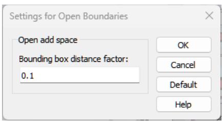
text_image
Settings for Open Boundaries Open add space Bounding box distance factor: 0.1 OK Cancel Default HelpThe size of this extra space is the length of the bounding box diagonal times the user defined factor, in our case 0.1. This value is also defined in the Particle Dynamics template. Click Cancel to leave this setting unchanged. Click Cancel again to leave the Boundary Conditions dialog box.
Note: There are two ways to create some space (background material) between structure and boundaries. The first way is described above. Alternatively, some extra space can be defined in the Background Properties dialog box. You can have a look in the paragraph Define the Background Material.
Start the Simulation
After having defined all necessary parameters, you are ready to perform your first simulation. The simulation is started from within the particle tracking solver control dialog box: Simulation: Solver Setup Solver .
text_image
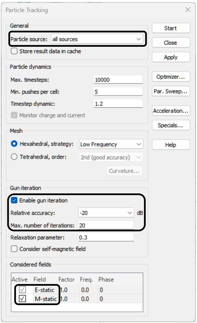
Particle Tracking General Particle source: all sources Store result data in cache Start Close Apply Particle dynamics Max. timesteps: 10000 Min. pushes per cell: 5 Timestep dynamic: 1.2 Optimizer... Par. Sweep... Acceleration... Specials... Mesh Hexahedral, strategy: Low Frequency Tetrahedral, order: 2nd (good accuracy) Curvature... Help Gun iteration Enable gun iteration Relative accuracy: -20 dB Max. number of iterations: 20 Relaxation parameter: 0.3 Consider self-magnetic field Considered fields Active Field Factor Freq. Phase ✓ E-static 1.0 0.0 0 ✓ M-static 1.0 0.0 0In this dialog box you can specify the settings of the Particle Tracking Solver and start the simulation process. If multiple particle sources are defined, you can choose between a simulation where all sources emit particles and a simulation where only a single source is active. Enable the Enable gun iteration option to activate the iterative gun solver algorithm, set the Relative accuracy to be -20 dB and the Max. number of iterations to 20. Thus, the Particle Tracking Solver does not just track the particles once through the computational domain. Instead, the solver iteratively repeats an electrostatic calculation and then tracks the particles until the desired accuracy of the space charge deviation between two successive iterations is reached.
The Considered fields box lists all electromagnetic fields that are available for the Particle Tracking Solver. In order to consider a specific field type for the tracking process, check the respective Active checkbox, in our case for the E- and the M-Static fields.
Now you can start the simulation procedure by clicking the Start button in the particle tracking dialog box. A few progress bars will appear to keep you up to date with the solver’s progress.
As you can see in the next paragraph, the complete solving procedure consists of three to four parts, depending upon the selected post processing steps. In this example, part two (electrostatic solver) and part three (particle tracking) are repeated iteratively until the relative accuracy condition specified in the gun iteration section is reached.
1. Magnetostatic Solver
1.1. Checking model: During this step, your input model is checked for errors such as invalid overlapping materials, etc.
1.2. Calculating matrices: During these steps, the system of equations, which will subsequently be solved, is set up.
1.3. Magnetostatic solver is running: During this stage, a linear equation solver calculates the field distribution inside the structure.
2. Electrostatic Solver
2.1. Calculating matrices: During these steps the system of equations, which will subsequently be solved, are set up.
2.2. Electrostatic solver is running: During this stage, a linear equation solver calculates the field distribution inside the structure.
3. Particle Tracking
3.1. Initializing Tracking Solver: The data structure for the collision detection of particles with solids is constructed.
3.2. Tracking Solver is running: The particles are emitted and tracked through the computational domain.
4. Post Processing
4.1. From the field distribution, additional results like the inductance matrix or the energy within the computational domain can be calculated.
After a few repetitions of steps two and three, the desired accuracy of -20 dB of the gun iteration is reached, i.e. the relative difference of the space charge distribution between two consecutive solver runs is less than -20 dB. The following diagram explains the algorithm of the iterative gun solver and its convergence condition:
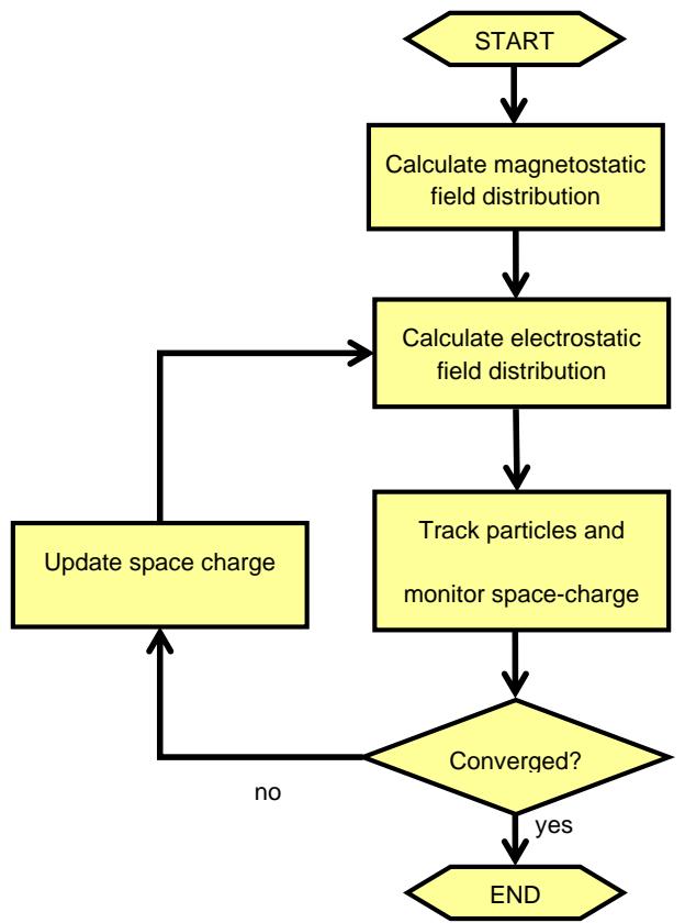
flowchart
graph TD
  START["START"] --> A["Calculate magnetostatic field distribution"]
  A --> B["Calculate electrostatic field distribution"]
  B --> C["Track particles and monitor space-charge"]
  C --> D{"Converged?"}
  D -->|no| E["Update space charge"]
  E --> B
  D -->|yes| END["END"]
Analyze the Results
In tracking applications, users are often interested in the particle beam behavior. To get an overview of the particle movement, a 3D visualization of the trajectories is available in the navigation tree NT: 2D/3D Results Trajectories. The trajectories should now look like in the following picture:
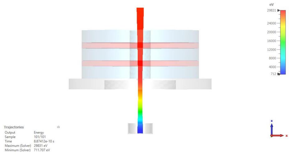
heatmap
| Metric | Value | | --- | --- | | Trajectories | — | | Output | Energy | | Sample | 101/101 | | Time | 8.87412e-10 s | | Maximum (Solver) | 29831 eV | | Minimum (Solver) | 711.707 eV |Colors indicate the particle energy. There are lots of options to modify this plot using the Particle Plot properties dialog box 2D/3D Plot: Plot Properties Properties .
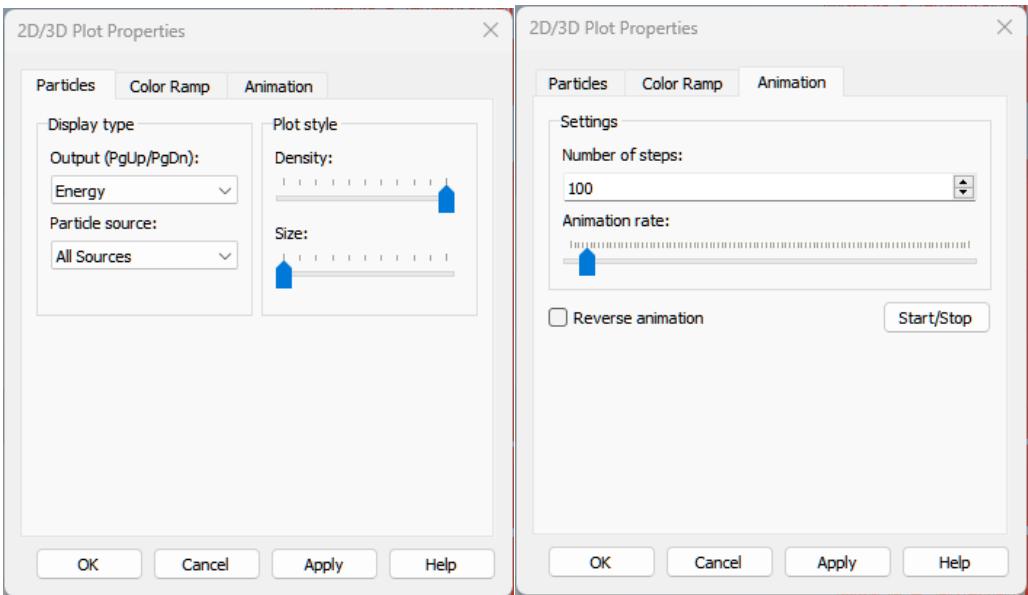
Open the dialog box and change some settings, for example the Display type. Click the Start/Stop button on the Animation tab to see the movement of the particles. Detailed explanations can be obtained from the online help. Click the Help button to open the online help. If you like to close this dialog box, click the Cancel button.
Field plots are also available in the navigation tree. To obtain the current density of the particle beam select NT: 2D/3D Results Particle Current Density in the navigation tree. To enable logarithmic scaling check the respective box at 2D/3D Plot Color Ramp Log.
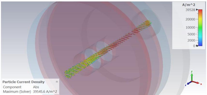
surface_3d
| Metric | Value | | --- | --- | | Component | Abs | | Maximum (Solver) | 39545.6 A/m^2 |Further plot settings can be changed in the 3D Vector Plot dialog box. This can be opened as usual via 2D/3D Plot: Plot Properties Properties .
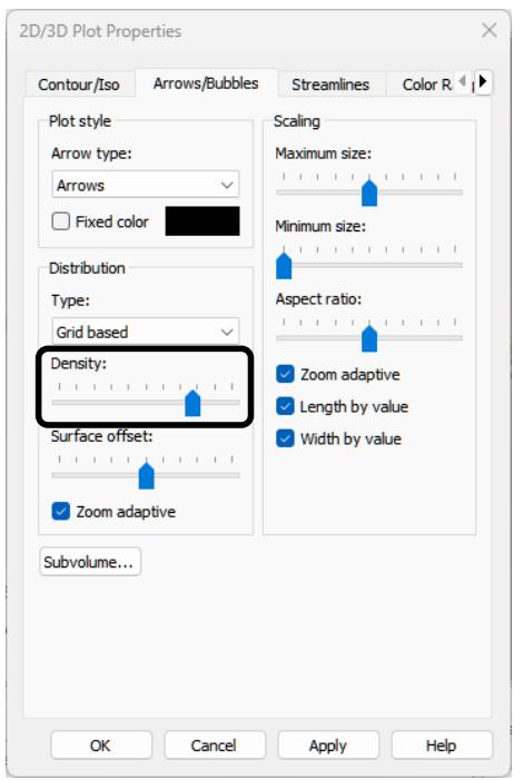
text_image
2D/3D Plot Properties Contour/Iso Arrows/Bubbles Streamlines Color R... Plot style Arrow type: Arrows Fixed color Distribution Type: Grid based Density: Surface offset: Zoom adaptive Subvolume... Scaling Maximum size: Minimum size: Aspect ratio: Zoom adaptive Length by value Width by value OK Cancel Apply HelpTo create the field plot above, the Density slider on the Arrows/Bubbles tab was shifted to the right. Try to change some settings. Click the OK button to leave this dialog box.
In the case of gun simulations with space charge limited emission, the emitted current is an important parameter. The 1D result plot emitted current versus gun iteration NT: 1D Results Particle Sources Current vs. Iteration particle1 is available in the navigation tree:
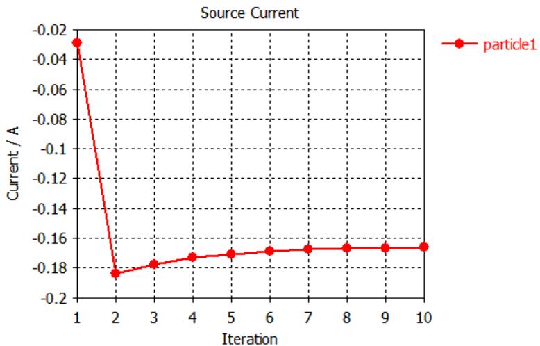
line
| Iteration | Current / A | | --- | --- | | 1 | -0.03 | | 2 | -0.184 | | 3 | -0.177 | | 4 | -0.172 | | 5 | -0.170 | | 6 | -0.169 | | 7 | -0.168 | | 8 | -0.167 | | 9 | -0.167 | | 10 | -0.167 |This 1D result offers you the possibility to control the emission process. Thus, it is very helpful that this plot is already available during the gun iteration.
Another plot is also available during the gun iteration, the gun code accuracy. If the user defined accuracy is reached, the iterative gun solver stops. To get this 1D result plot select the folder NT: 1D Results Convergence Gun Iteration Charge Accuracy in the navigation tree:
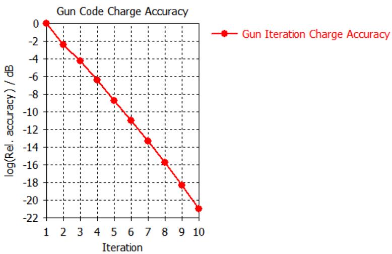
line
| Iteration | log(Rel. accuracy) / dB | | --- | --- | | 1 | 0 | | 2 | ~-2.3 | | 3 | ~-4.2 | | 4 | ~-6.3 | | 5 | ~-8.7 | | 6 | ~-10.9 | | 7 | ~-13.3 | | 8 | ~-15.7 | | 9 | ~-18.3 | | 10 | ~-20.9 |Apart from this 1D graph, the development of the emitted charge and the perveance during the gun iteration process are also available via NT: 1D Results Particle Sources Charge vs. Iteration particle1 and NT: 1D Results Particle Sources Perveance vs. Iteration particle1.
The collision information under NT: 1D Results Total Collision Information can also be very interesting, because these graphs contain e.g. information about the power that is absorbed by a solid. Precise numbers can easily be read from these graphs via the entry Show Axis Marker from the context menu:
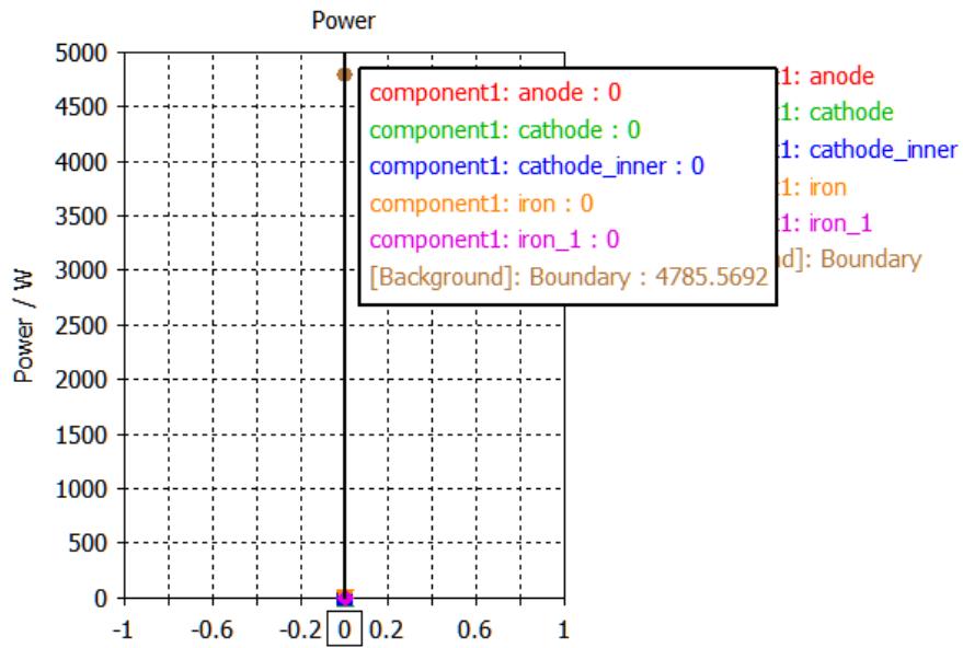
scatter
| Component | Power (W) | | --- | --- | | anode | 0 | | cathode | 0 | | cathode_inner | 0 | | iron | 0 | | iron_1 | 0 | | Boundary | 4785.5692 |In this case the background consists of vacuum, thus all particles are absorbed by the boundary of our calculation domain.
Parameterization of the Model
The previous steps demonstrated how to enter and analyze a simple structure. However, structures are usually analyzed to improve their performance. This procedure may be called “design” in contrast to the “analysis” done before.
After you get some information on how to improve the structure, you will learn how to optimize the structure’s parameters. This could be done by modifying each parameter manually, but this of course is not the best solution. CST Studio Suite offers various options to describe the structure parametrically in order to change the parameters easily.
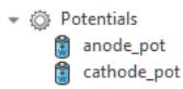
Let us assume you are interested in the dependency of the emitted current on the cathode's potential. To obtain this dependency, first of all the potential has to be parameterized. Thus, double click on the potential NT: Potentials cathode_pot in the navigation tree.
The Edit Potential dialog box opens and the potential can be edited. Instead of a number type the string "phi" in the Potential value field.
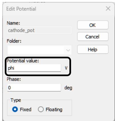
text_image
Edit Potential Name: cathode_pot Folder: Potential value: phi V Phase: 0 deg Type Fixed FloatingIf you click the OK button, you will be asked to delete the current results. Just click the OK button to delete the results. Then the dialog box New Parameter opens to define the value of your parameter "phi".
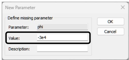
text_image
New Parameter Define missing parameter Parameter: phi Value: -3e4 Description:Enter a value of -3e4 and click the OK button. You have successfully defined your first parameter. The values of your parameters can be edited and checked in the Parameter List window that is usually located in the lower left part of the main window:
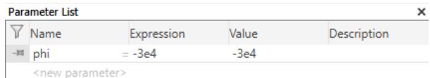
text_image
Parameter List Name Expression Value Description phi = -3e4 -3e4Since we did not change the value of the cathode's potential, the results of the simulation would be the same. We will now change the setup to run a so called Parameter Sweep to get the emitted current for potentials in the range from -32 kV to -28 kV. To do this, open the Particle Tracking solver dialog box Simulation: Solver Setup Solver .
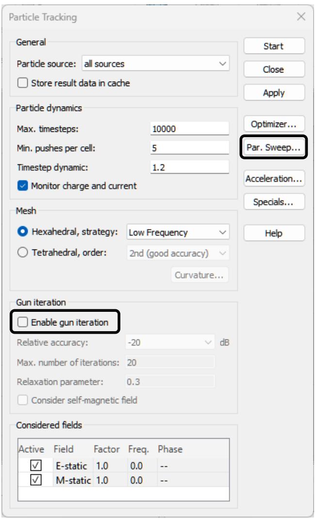
text_image
Particle Tracking General Particle source: all sources □ Store result data in cache Particle dynamics Max. timesteps: 10000 Min. pushes per cell: 5 Timestep dynamic: 1.2 ✓ Monitor charge and current Mesh ● Hexahedral, strategy: Low Frequency ○ Tetrahedral, order: 2nd (good accuracy) Curvature... Gun iteration □ Enable gun iteration Relative accuracy: -20 dB Max. number of iterations: 20 Relaxation parameter: 0.3 □ Consider self-magnetic field Considered fields Active Field Factor Freq. Phase ✓ E-static 1.0 0.0 -- ✓ M-static 1.0 0.0 -- Start Close Apply Optimizer... Par. Sweep... Acceleration... Specials... HelpTo save some time during the parameter sweep disable the checkbox Enable gun iteration. The tracking solver will now run only one calculation and will not operate in the iterative mode.
Click the button Par. Sweep to open the dialog box Parameter Sweep and to configure the parameter range and also the expected results of the parameter sweep.
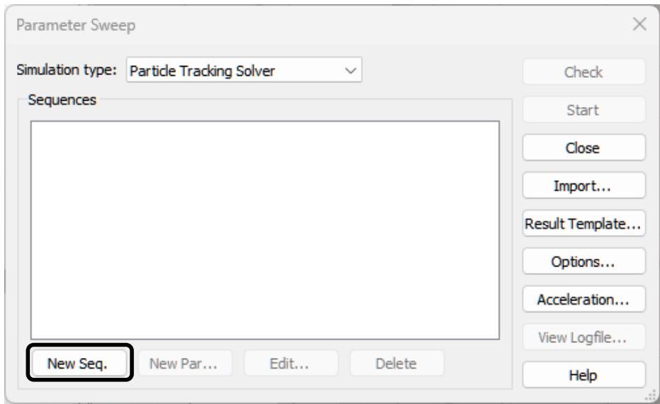
text_image
Parameter Sweep Simulation type: Particle Tracking Solver Sequences New Seq. New Par... Edit... Delete Check Start Close Import... Result Template... Options... Acceleration... View Logfile... HelpIn this dialog box you can specify calculation sequences that consist of various parameter combinations. To add such a sequence, click the New Seq. button now. Then click the New Par button to add a parameter variation to the sequence:
text_image
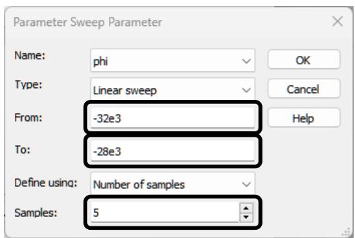
Parameter Sweep Parameter Name: phi Type: Linear sweep From: -32e3 To: -28e3 Define using: Number of samples Samples: 5In the resulting dialog box you can select the name of the parameter to vary in the Name field. Then you can specify different sweep types to define the sampling of the parameter space (Linear sweep, Logarithmic sweep, Arbitrary points). Depending on this selection the sampling can be defined further, e.g. the linear sweep option allows us to define the lower (From) and upper (To) bounds for the parameter variation as well as the definition of either the number of samples or the step width.
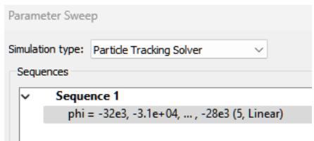
In this example you should perform a linear sweep from -32 kV to -28 kV in 5 steps. Click the OK button to confirm your changes. The definition of the sequence is finished but we still need to configure the expected result, the emitted current. The parameter sweep dialog box should look as follows:
text_image
Parameter Sweep Simulation type: Particle Tracking Solver Sequences ✓ Sequence 1 phi = -32e3, -3.1e+04, ..., -28e3 (5, Linear)After a successful simulation run, many simulation results are already generated automatically under NT: 1D Results and saved in the parametric storage. For more detailed investigations and customized evaluations, Template Based Post-Processing is available. Often, the parametric results are already sufficient to analyze the results.
However, the general procedure of defining and handling Result Templates is outlined below.
In order to evaluate a particular quantity of interest during the parameter sweep, it needs to be defined in advance. Here, the current emitted from the particle source should be monitored.
As can be seen above, this quantity is available as a plot versus gun iteration number under NT: 1D Results Particle Sources Current vs. Iteration particle1. For finding the final value obtained during the gun iteration, we have to extract the value that corresponds to the rightmost point in the plot. Note that this approach is also valid if Gun iteration is deactivated, as we did above, since then the plot only contains a single point.
In order to define the results of interest, click on the button Result Template. The Template Based Post-Processing dialog box opens. Templates are separated into several Template Groups.
text_image
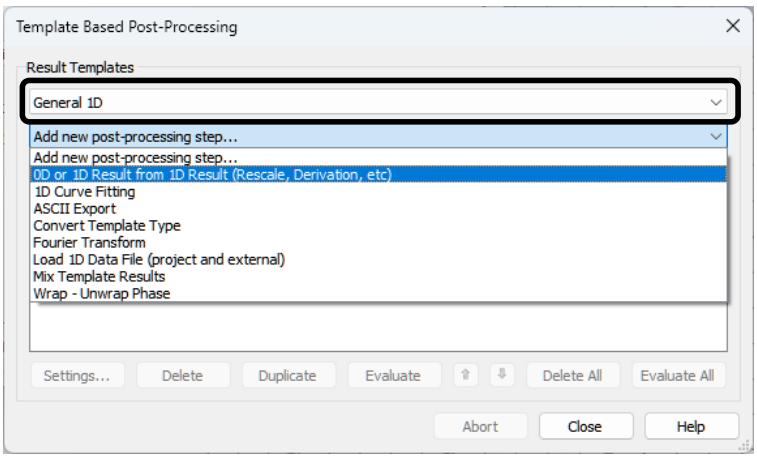
Template Based Post-Processing Result Templates General 1D Add new post-processing step... Add new post-processing step... 0D or 1D Result from 1D Result (Rescale, Derivation, etc) 1D Curve Fitting ASCII Export Convert Template Type Fourier Transform Load 1D Data File (project and external) Mix Template Results Wrap - Unwrap PhaseChoose the template 0D or 1D Result from 1D Result (Rescale Derivation, etc) in the General 1D group. This very powerful template is intended for post processing or extracting data from any 1D plot. Once you choose this template, a dialog box opens where the data source and the operation have to be entered.
text_image
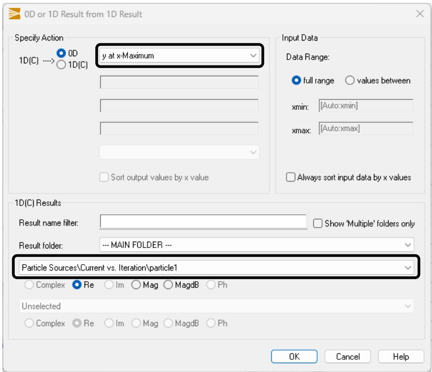
0D or 1D Result from 1D Result Specify Action 1D(C) ---> 0D y at x-Maximum 1D(C) Input Data Data Range: full range values between xmin: [Auto:xmin] xmax: [Auto:xmax] Always sort input data by x values Sort output values by x value 1D(C) Results Result name filter: Show 'Multiple' folders only Result folder: --- MAIN FOLDER --- Particle Sources\Current vs. Iteration\particle1 Complex Re Im Mag MagdB Ph Unselected Complex Re Im Mag MagdB Ph OK Cancel HelpUnder Specify Action select y at x-Maximum. Under 1D(C) Results, the data source has to be selected – in our case Particle Sources\Current vs. Iteration\particle1. Leave the dialog by pressing OK.
The Template Based Post-Processing dialog box should be still open and contain the following row:
| Result name | Type | Engine | Template name | Value | Active On/Off | |
| 1 | particle1_0D_yAtXMax | 0D-P | VBA | 0D or 1D Result from ... | On (Paramel √ |
The Result name can be changed by clicking onto the respective cell. You should change it to something more recognizable since this will become the result plot title, choose, “Emitted Current”:
| Result name | Type | Engine | Template name | Value | Active On/Off | |
| 1 | Emitted Current | 0D-P | VBA | 0D or 1D Result from ... | On (Paramel √ |
Click the Close button to return to the parameter sweep. Now start the parameter sweep by clicking Start. After confirming the request to delete existing results with OK, the calculation may take a few minutes. The navigation tree contains a new item called Tables from which you can select the item NT: Tables 0D Results Emitted Current. The 1D result plot should look like in the picture below and gives you the relation between input voltage and emitted current of the electron gun:
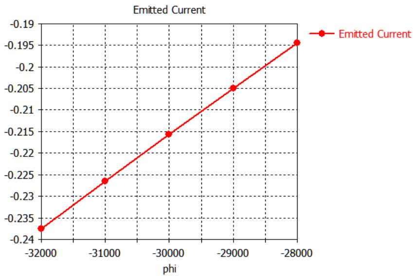
line
| phi | Emitted Current | | --- | --- | | -32000 | -0.237 | | -31000 | -0.226 | | -30000 | -0.215 | | -29000 | -0.205 | | -28000 | -0.194 |Automatic Optimization of the Structure
Let us assume that you wish to adjust the emitted current to a value of -0.22 A (which can be achieved within the parameter range of -32 kV to -30 kV according to the parameter sweep). Figuring out the proper parameter can be a lengthy task, but it can also be performed automatically.
CST Studio Suite offers a very powerful built-in optimizer feature for such parametric optimizations.
To use the optimizer, open the tracking solver control dialog box Simulation: Solver Setup Solver in the same way as before, or directly via Simulation: Solver Optimizer . Click the Optimizer button to open the optimizer control dialog box.
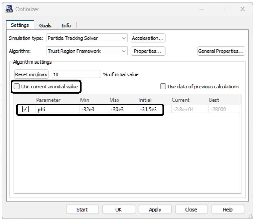
text_image
Optimizer Settings Goals Info Simulation type: Particle Tracking Solver Acceleration... Algorithm: Trust Region Framework Properties... General Properties... Algorithm settings Reset min/max 10 % of initial value Use current as initial value Use data of previous calculations Parameter Min Max Initial Current Best ✓ phi -32e3 -30e3 -31.5e3 -2.8e+04 -28000 Start OK Apply Close HelpFirst, activate the desired parameter(s) for the optimization in the Settings Tab of the optimization dialog box, here the parameter "phi" should be checked. Second, specify the minimum and maximum values for this parameter during the optimization. From the parameter sweep, we already know that the searched potential is greater than -32 kV and lower than -30 kV. Therefore, you can enter a parameter range between -32 kV and -30 kV. Deactivate Use current as initial value and set the initial start value for the optimization, e.g. to -31.5 kV.
For this simple example, the other settings can be kept as default. Refer to the online documentation for more information on these settings. You can specify a list of goals you wish to achieve during the optimization. In this example, the objective is to find a parameter value for which the emitted current becomes -0.22 A. The next step is to specify this optimization goal. Switch to the Goals Tab and click Add New Goal.
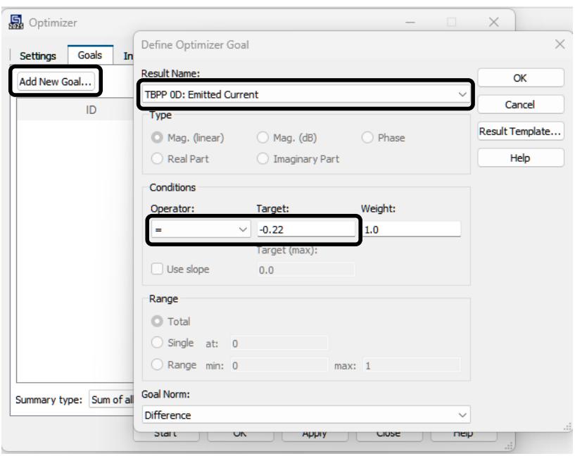
text_image
Add New Goal... Define Optimizer Goal Result Name: TBPP 0D: Emitted Current OK Cancel Real Part Mag. (linear) Mag. (dB) Phase Imaginary Part Results Template... Help Conditions Operator: Target: Weight: = -0.22 1.0 Target (max): Use slope 0.0 Range Total Single at: 0 Range min: 0 max: 1 Goal Norm: Difference Summary type: Sum of all Start OK Apply Close HelpNow you can define the goal for the emitted current. Since you would like to find a value of -0.22 A, you should select the equal operator in the conditions frame. Then set the Target to -0.22. After you click OK, the optimizer dialog box should look as follows:
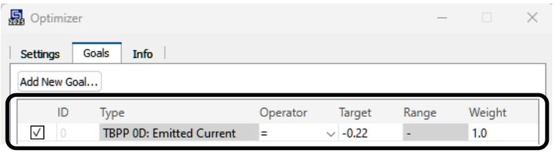
text_image
Optimizer Settings Goals Info Add New Goal... ID Type Operator Target Range Weight ✓ 0 TBPP 0D: Emitted Current = -0.22 - 1.0Note: The optimizer is capable of optimizing multiple parameters at once. Detailed information can be obtained from the online help.
Up to now, you have specified which parameters to optimize and set the goal that you want to achieve. The next step is to start the optimization procedure by clicking the Start button. As shown in the next picture, the optimizer will display its progress in an output window in the Info tab, which is activated automatically. After the whole process has finished, the optimizer output window contains the best parameter values in order to achieve the desired goal.
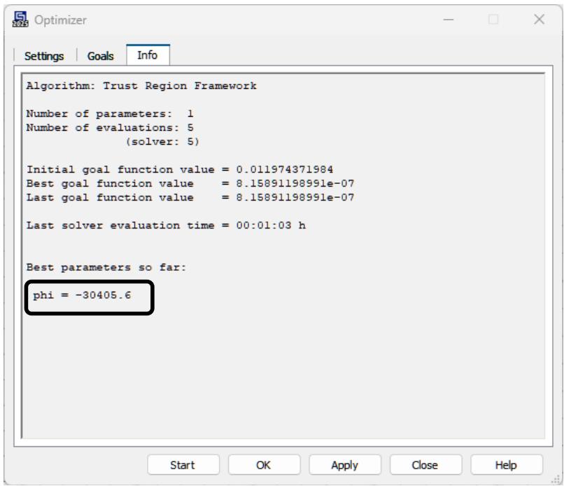
text_image
Algorithm: Trust Region Framework Number of parameters: 1 Number of evaluations: 5 (solver: 5) Initial goal function value = 0.011974371984 Best goal function value = 8.15891198991e-07 Last goal function value = 8.15891198991e-07 Last solver evaluation time = 00:01:03 h Best parameters so far: phi = -30405.6Note that, due to sophisticated optimization technology, only five solver runs are necessary to find the optimal solution with very high accuracy.
Click the Close button to leave the dialog box. Now look at the final result of the emitted current for the optimal parameter setting phi = -30405.6 V by clicking NT: 1D Results Particle Sources Current vs. Iteration. You should obtain the following result:
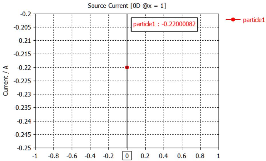
scatter
| Series | X | Current (A) | | --- | --- | --- | | particle1 | 0 | -0.2200082 |As you can see, the final emitted current for the optimized voltage parameter is -0.22 A as it was previously defined by the setting of the optimization goal.
Additional Information: More settings for the Particle Tracking Solver
The Particle Tracking and the Particle Tracking Specials dialog boxes offer many more options to change the solver properties. The latter is available by selecting Simulation: Solver Setup Solver and clicking the Specials button.
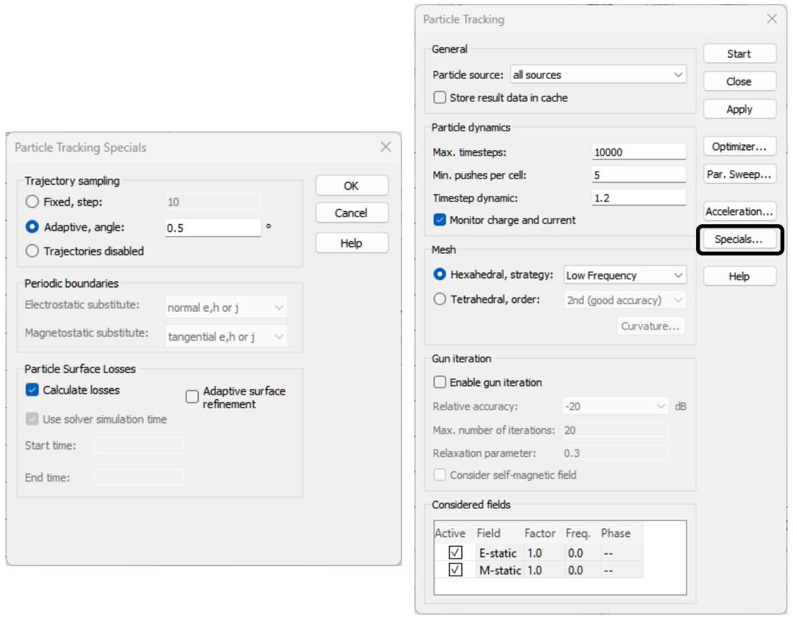
The Particle dynamics frame offers the possibility to change specific settings of the particle tracking algorithm. The setting Max. timesteps defines the maximum number of simulated steps performed by the tracking algorithm. The Min. pushes per cell value determines the spatial sampling rate of the particle trajectories. The Timestep dynamic parameter specifies the variation of the time step between two pushes and introduces a dynamic adaptation of the time step to the highest particle velocity. Activating the checkbox Monitor charge and current results in monitoring the space charge and current density generated by the particles. This is automatically activated for gun iteration simulations.
In the Gun iteration frame, in addition to the desired Relative accuracy, the maximum number of iterations of consecutive electrostatic simulations and particle tracking computations is defined. The Relaxation parameter describes the influence of the last obtained space charge distribution to the overall charge distribution, which is considered in the next electrostatic computation. By checking Consider self-magnetic field, the magnetic field generated by the particles can be included in the gun iteration.
In order to save disk space, the trajectory data is usually not written for every time step. Instead, a subsampling is performed. The sampling method and its parameters can be set in the Trajectory sampling section of the Particle Tracking Specials dialog.
Additional Information: Treating PEC as Normal Material for Magnetostatic
Computations
Simulation Setups used for Particle Tracking or PIC simulations often consist of a metallic beam pipe or similar enclosing structure. If these structures are modeled using PEC material, they effectively cannot be penetrated by magnetic fields, which is physically correct within the simulation model but usually not desired.
This is why it is possible to treat PEC as a normal material for the Magnetostatic Solver via a setting in its Specials dialog.
The option Consider PEC as Normal is default only when a Particle Tracking or PIC project template is used - otherwise this checkbox is disabled by default. If you want to change or check this setting, open the Special Settings dialog box of the Magnetostatic Solver Parameters via Home: Simulation Setup Solver (dropdown list) M-Static Solver, Home: Simulation Setup Solver Specials.
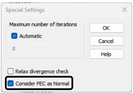
text_image
Special Settings Maximum number of iterations ✓ Automatic 0 OK Cancel Help ☐ Relax divergence check ✓ Consider PEC as NormalIf the checkbox Consider PEC as Normal is enabled, PEC materials are considered like normal materials with a permeability µ which can be defined in the material properties of the PEC material. In case the solver is started from problem class “Tracking”, this setting is activated automatically.
Please note that in stand-alone magnetostatic simulations using the Problem Type “Low Frequency”, different results compared to Problem Type “Particle” are obtained despite otherwise identical settings due to the different defaults regarding the consideration of PEC type materials.
Additional Information: Using tetrahedral meshes in the Tracking Solver
Especially for models with curved surfaces in the vicinity of the particle beam, a representation of the structure by a hexahedral mesh may require a large number of cells. In these cases, it can be helpful to use a tetrahedral mesh that will model the structure’s surfaces more naturally and thus can yield more accurate surface fields.
You can either switch to the tetrahedral mesh type by selecting Simulation: Mesh Global Properties (dropdown list) Tetrahedral and pressing OK in the appearing Mesh Properties dialog or alternatively via the option in the solver setup dialog Simulation: Solver Setup Solver Mesh Tetrahedral.
When changing the mesh, you will be informed that any existing results have to be deleted. Confirm the deletion of the results by clicking OK.
Before starting a new simulation based on a tetrahedral mesh, a few settings in the model setup have to be changed, part of which can be seen as general recommendations for using the tetrahedral tracking solver:
Open boundaries are not supported. They are automatically replaced by magnetic boundaries (Ht = 0) upon solver start.
In many cases, the automatically generated mesh will be a good starting point for performing your simulations. However, in order to obtain a mesh well adapted to the simulation type, some settings should be changed.
o For modifying the global mesh resolution, you can set the mesh properties via Mesh Global Properties . In the mesh properties dialog, enter 10 under Cells per max model box edge for Model and 15 for Background.
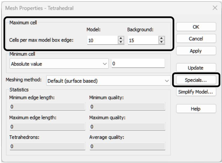
text_image
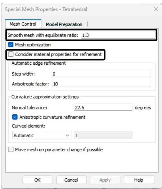
Mesh Properties - Tetrahedral Maximum cell Model: Background: Cells per max model box edge: 10 15 Minimum cell Absolute value 0 Meshing method: Default (surface based) Statistics Minimum edge length: Minimum quality: 0 0 Maximum edge length: Maximum quality: 0 0 Tetrahedrons: Average quality: 0 0 OK Cancel Apply Update Specials... Simplify Model... Helpo As the particles only interact with the electromagnetic fields in the vacuum regions, a mesh refinement of the permanent magnets is not of the highest priority. Therefore, you may disable the checkbox Consider material properties for refinement in the Specials dialog. Moreover, the value in the edit field Smooth mesh with equilibrate ratio should be set to 1.3 in order to avoid generating a too large number of tetrahedrons for this example.
text_image
Special Mesh Properties - Tetrahedral Mesh Control Model Preparation Smooth mesh with equilibrate ratio: 1.3 ✓ Mesh optimization □ Consider material properties for refinement Automatic edge refinement Step width: 0 Anisotropic factor: 10 Curvature approximation settings Normal tolerance: 22.5 degrees ✓ Anisotropic curvature refinement Curved element: Automatic 1 □ Move mesh on parameter change if possible OK Cancel Apply HelpDue to using the project template for setting up the simulation project, most of these settings have already been applied automatically.
The mesh can be visualized by entering the mesh view Home: Mesh Mesh View and then pressing Mesh: Mesh Update to invoke the tetrahedral mesher. In case you do not trigger the mesh generation manually, the mesh is automatically constructed upon solver start. After a few seconds, the mesh appears. For the structure in this example, it looks as follows:
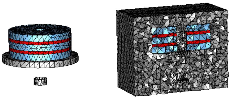
The right image has been generated using Mesh: Visibility Background and Mesh: Sectional View Cutting Plane . It includes a visualization of the background mesh cells, i.e., the free-space region where the particle trajectories will be computed. Naturally, the mesh quality in the beam region is important for achieving accurate results.
Please note that particle tracking simulations that are using a tetrahedral mesh will in general be slower than simulations with the same number of hexahedral cells. However, since tetrahedral meshes yield a more precise surface representation, a considerably smaller number of cells will often be sufficient for getting accurate results.
Press Update in the Mesh Properties dialog. This requests the tetrahedral mesher to update the mesh representation. The total number of tetrahedrons is close to 55,000 now, as can be seen in the status bar:

As in the hexahedral case, a local control of the mesh resolution can be reached via the local mesh properties of the respective component.
After leaving the mesh inspection mode via Mesh: Close Close Mesh View , you could start the simulation as before using the particle tracking solver control dialog box: Simulation: Solver Setup Solver Start. However, due to some restrictions that apply to the tracking solver when used with tetrahedral meshes, the following preparations have to be performed (if you omit these steps, the solver will emit respective messages to guide you towards solving possible issues):
While being relative to the mesh dimensions in the hexahedral case, the emission distance for the space charge limited emission model has to be an absolute value when using a tetrahedral mesh. In general, it is a good idea to review all settings of the particle source after switching the mesh type.
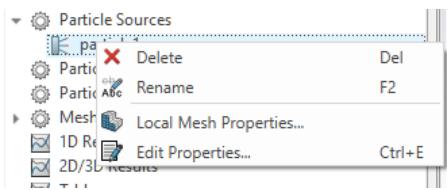
In order to do so, right-click onto the particle source in the navigation tree NT: Particle Sources particle1 and select Edit Properties… from the context menu.
text_image
Particle Sources Delete Del Partic Rename F2 Mesh Local Mesh Properties... 1D RecThis will open the Edit Particle Area Source dialog again. Here you should increase the Number of emission points to a value around 400 again by setting the Scale Factor to 10 and adjusting the slider appropriately.
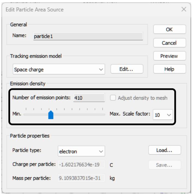
text_image
Edit Particle Area Source General Name: particle1 OK Cancel Preview Help Tracking emission model Space charge Edit... Emission density Number of emission points: 410 Adjust density to mesh Min. Max. Scale factor: 10 Particle properties Particle type: electron Load... Charge per particle: -1.602176634e-19 C Save... Mass per particle: 9.1093837015e-31 kgFurthermore, open the settings of the emission model using the Edit button in the Tracking emission model frame, check the settings and press OK twice to close both dialogs.
Finally, you can now run the particle tracking solver with a tetrahedral mesh via its solver control dialog box: Simulation: Solver Setup Solver Start.
The results should look similar to the ones obtained using a hexahedral mesh for the workflow example described earlier in this section (here for phi = -30 kV and active gun iteration again):
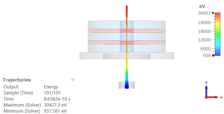
heatmap
| Metric | Value (eV) | | --- | --- | | Maximum (Solver) | 30427.3 | | Minimum (Solver) | 937.581 | | Sample (Time) | 101/101 | | Time | 8.6382e-10 s |Summary
This example gave you a basic overview of the key concepts of the Tracking Solver of CST Studio Suite. You should now have a good idea of how to do the following:
- Create a structure using the solid modeler
- Specify the solver parameters, check and modify the mesh and start the tracking simulation
- Visualize the electromagnetic field distributions and the particles trajectories
- Define a structure using parameters
- Use the parameter sweep tool for parameter studies
- Perform automatic optimizations
If you are familiar with all these topics, you have a very good starting point for further improving your usage of CST Studio Suite.
For more information on a particular topic, we recommend that you look at the contents page of the online help manual, which can be opened via File: Help Help Contents – Get Help using CST Studio Suite . If you have any further questions or remarks, do not hesitate to contact our technical support team. We also strongly recommend that you participate in one of our special training classes held regularly at a location near you. Please ask us for details.
Simulation Workflow: Electromagnetic Particle-in-Cell
The basic procedure of running the electromagnetic (EM) particle-in-cell (PIC) solver is very similar to the one demonstrated in the tracking simulation workflow. In contrast to the tracking solver, particles and electromagnetic fields are computed in a selfconsistent way using a time integration scheme. For more information on the physics that can be modelled with the EM PIC solver, an overview is provided in Chapter 3 – Solver Overview: Particle-in-Cell Solver.
The following example demonstrates how to perform a PIC calculation for a simple output cavity of a klystron. Studying this example carefully will allow you to become familiar with many standard operations that are necessary to perform a PIC simulation within CST Studio Suite.
Go through the following explanations carefully even if you are not planning to use the software for PIC simulations. Only a small portion of the example is specific to this particular application type since most of the considerations are general to all solvers and application domains.
The following explanations always describe the menu-based way to open a particular dialog box or to launch a command. Whenever available, the corresponding toolbar item is displayed next to the command description. Due to the limited space in this manual, the shortest way to activate a particular command (i.e. by pressing a shortcut key or activating the command from the context menu) is omitted. You should regularly open the context menu to check available commands for the currently active mode.
The Structure
This workflow example demonstrates how to build up the output cavity of a klystron for a PIC simulation. A klystron is a device to amplify microwave and/or radio frequency signals. The output resonator is the last stage (cavity) of a klystron. The amplified signal can be extracted using waveguide ports.
Since only the output resonator as a part of the klystron is simulated, a Gaussian emission model is used to define an already bunched particle beam.
natural_image
3D mechanical component diagram showing a central shaft and two cylindrical ports (no text or symbols)CST Studio Suite allows you to define the properties of the background material. Background material is considered for the space in which no shape is defined. For this structure, it is sufficient to use vacuum for the klystron cavity and perfect electrical conductor (PEC) for the surrounding background space.
Create a New Project
After launching the CST Studio Suite you will enter the start screen showing you a list of recently opened projects and allowing you to select the application that best suits your requirements. The easiest way to get started is to configure a project template, which defines the basic settings that are important for your typical application. Therefore, click on the New Template button in the New Project from Template section within the New and Recent tab.
Next, you should choose the application area, Particle Dynamics for the example in this tutorial, and then select the workflow by double-clicking on the corresponding entry.
flowchart
graph LR
  A["Microwaves & RF/OPTAL"] --> B["EDA/ELECTRONICS"]
  B --> C["EMC/EMI"]
  C --> D["Particle Dynamics"]
  D --> E["Static/Low Frequency"]
  E --> F["Precipitation"]
  F --> G["Space Applications"]
  G --> H["Vacuum Electronic Devices"]
  H --> I["Accelerator Components"]
  I --> J["Beam Optics"]
Please then select the following workflow: Vacuum Electronic Devices Klystron Hot Test Particle in Cell .
You are then requested to select the units that fit your application best. For this example, please select the dimensions as follows:
| Dimensions: | mm |
| Frequency: | GHz |
| Time: | ns |
| Temperature: | Kelvin |
For the specific application in this tutorial, the other settings can be left unchanged. After clicking the Next button, you can give the project template a name and review a summary of your initial settings:
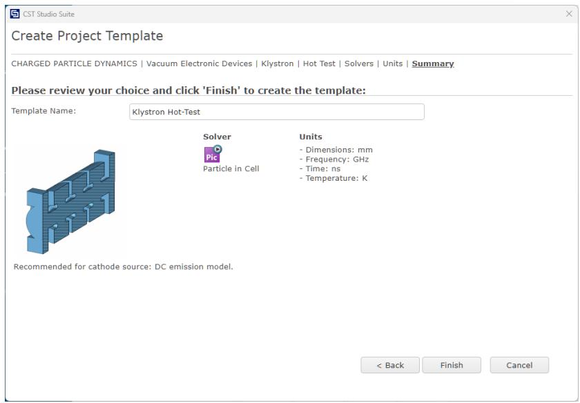
text_image
Create Project Template CHARGED PARTICLE DYNAMICS | Vacuum Electronic Devices | Klystron | Hot Test | Solvers | Units | Summary Please review your choice and click 'Finish' to create the template: Template Name: Klystron Hot-Test Solver Units Pic - Dimensions: mm Particle in Cell - Frequency: GHz - Time: ns - Temperature: K Recommended for cathode source: DC emission model. < Back Finish CancelFinally, click the Finish button to save the project template and to create a new project with the appropriate settings. CST Studio Suite for Particle Dynamics Simulation will be launched automatically due to the choice of this specific project template within the application area Particle Dynamics. Save the newly created “Untitled” project on your hard disk using a name of your choice.
Please note: When you click again on the File: New and Recent you will see that the recently defined template appears below the Project Templates section. For further projects in the same application area, you can simply click on this template entry to launch CST Studio Suite for Particle Dynamics Simulation with useful basic settings. It is not necessary to define a new template each time. You are now able to start the software with reasonable initial settings quickly with just one click on the corresponding template.
Please note: All settings made for a project template can be modified later on during the construction of your model. For example, the units can be modified in the units dialog box (Home: Settings Units ) and the solver type can be selected in the Home: Simulation Setup Solver drop-down list.
Open the PIC QuickStart Guide
An interesting feature of the online help system is the QuickStart Guide, an electronic assistant that will guide you through your simulation. If it does not show up automatically, you can open this assistant by selecting QuickStart Guide from the Help button in the upper right corner.
The following dialog box should then be visible at the upper right corner of the main view:
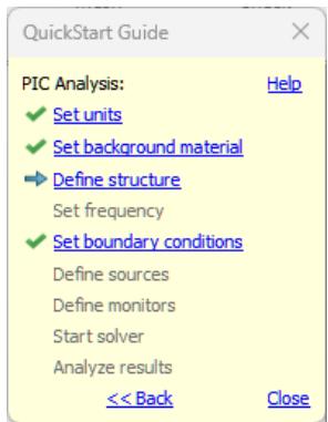
text_image
QuickStart Guide PIC Analysis: ✓ Set units ✓ Set background material → Define structure Set frequency ✓ Set boundary conditions Define sources Define monitors Start solver Analyze results << Back Help CloseAs the project template has already set the solver type, units, boundary conditions and background material, the PIC Analysis is preselected and some entries are marked as done. The blue arrow always indicates the next step necessary for your problem definition. You do not have to follow the steps in this order, but we recommend you follow this guide at the beginning to ensure that all necessary steps have been completed.
Look at the dialog box as you follow the various steps in this example. You may close the assistant at any time. Even if you re-open the window later, it will always indicate the next required step.
If you are unsure of how to access a certain operation, click on the corresponding line. The QuickStart Guide will then either run an animation showing the location of the related menu entry or open the corresponding help page.
Define the Units
The Klystron Hot-Test template has already made some settings for you. The defaults for this structure type are geometrical values in mm and times in ns. You can change these settings by entering the desired settings in the units dialog box (Home: Settings Units ) but for this example you should just leave the settings as specified by the template. Additionally, the used units are also displayed in the status bar:

Define the Background Material
As discussed above in the Structure section, the klystron cavity is surrounded by perfect electrical conductor (PEC). The material type PEC is already set as default background material in the Klystron Hot-Test template. You may change the background material in the corresponding dialog box (Simulation: Settings Background ). For this example, no change of the background material is needed.
Model the Structure
Having defined the initial general settings, the 3D view window is now visible and the working plane is shown therein. The working plane can be turned off (and on) by clicking on View: Visibility Working Plane .
Then, you can start building the 3D structure. First, create a vacuum cylinder along the z-axis of the coordinate system using the following steps:
- Select the cylinder creation tool Modeling: Shapes Cylinder .
- Press the ESC key to open the dialog box. Do not click a point in the working plane.
- Enter "cavity" as name.
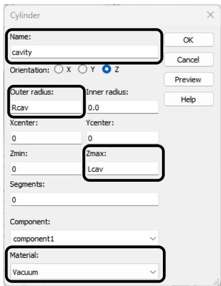
text_image
Cylinder Name: cavity Orientation: X Y Z Outer radius: Rcav Inner radius: 0.0 Xcenter: Ycenter: 0 0 Zmin: Zmax: 0 Lcav Segments: 0 Component: component1 Material: Vacuum- Enter the parameters "Rcav" as outer radius and "Lcav" as Zmax. Set the Material to "Vacuum". Click the OK button to confirm the changes.
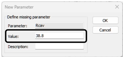
- The New Parameter dialog box appears. Enter 38.8 as value for Rcav. Press the Return key to confirm. It is also possible to add a description of the parameter.
text_image
New Parameter Define missing parameter Parameter: Rcav Value: 38.8 Description:- Another New Parameter dialog box appears. Enter 22 as value for Lcav. Press the Return key to confirm. The defined parameters are shown in the Parameter List window of the CST Studio Suite. To view the newly created shape, click on View: Change View Reset view .
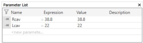
text_image
Parameter List Name Expression Value Description Rcav = 38.8 38.8 Lcav = 22 22natural_image
3D diagram of a red circular object with coordinate axes (x, y, z) and directional arrows indicating movement or orientation (no text or symbols)text_image
Cylinder Name: solid1 Orientation: ○ U ○ V ● W Outer radius: Rtub Inner radius: 0.0 Ucenter: Vcenter: 0 Wmin: 0 Wmax: Ltub Segments: 0 Component: component1 Material: Vacuum OK Cancel Preview Helptext_image
Diagram showing 3D coordinate system with labeled axes (x, y, z) and vectors (u, v, w) around a cylindrical object.text_image
Cylinder Name: solid2 Orientation: ○ U ○ V ● W Outer radius: Rtub Inner radius: 0.0 Ucenter: 0 Vcenter: 0 Wmin: 0 Wmax: Ltub Segments: 0 Component: component1 Material: Vacuum OK Cancel Preview Helpnatural_image
3D diagram of a mechanical component with a central flange and external shaft, showing directional arrows (no text or symbols)natural_image
3D rendered mechanical component with flange and cylindrical shaft (no text or symbols)text_image
Brick Name: solid3 Umin: -WW Vmin: -5 Wmin: 0 Component: component1 Material: Vacuum Umax: WW Vmax: 25 Wmax: Lcav OK Cancel Preview Helptext_image
Shape Intersection The new shape (highlighted) component1:solid3 (Vacuum) intersects with an old shape component1:cavity (Vacuum) Boolean combination None Insert highlighted shape Trim highlighted shape Add both shapes Intersect both shapes Cut away highlighted shape Apply to all intersections OK Cancel Helpnatural_image
3D diagram of a mechanical component with labeled axes (U, V) and a red vehicle, no readable text or symbols present.text_image
Transform Selected Object Operation Translate Scale Rotate Mirror Copy Unite Independent OK Cancel Apply Preview Reset Help Less << Repetitions Repetition factor: 1 Mirror plane normal X: 0 Y: 1 Z: 0 Mirror plane origin Shape center X0: 0 Y0: 0 Z0: 0 Change destination Component: Material: component1 Vacuumnatural_image
3D mechanical assembly diagram showing a central shaft with two cylindrical heads and a rectangular housing (no text or symbols)natural_image
3D mechanical component diagram showing a flanged housing with two cylindrical ports and a central shaft (no text or symbols)natural_image
3D mechanical part diagram with coordinate axes (x, y, z) and a red circular feature, no text or symbols present.text_image
Define Particle Circular Source General Name: particle1 PIC emission model Gauss Edit... Emission circle Use pick Invert picked normal Outer radius: Rtub*0.3 Inner radius: 0.0 Xcenter: #906710175e-15 Xnormal: 0 Ycenter: 0 Ynormal: 0 Zcenter: -55 Znormal: 1 Emission density Lines: 5 Emiss. points: 81 Radial dependency Constant Edit... Oblique emission settings Angle theta: 0.0 ° Angle phi: 0.0 ° Particle properties Type: electron Load... Charge: -1.602176634e-19 C Save... Mass: 9.1093837015e-31 kg| General | Kinetic | ||
| Setting | Value | Setting | Value |
| Charge (abs) | 50e-9 | Kinetic type | Gamma |
| Bunches | 15 | Kinetic value | 2 |
| Time / Length | Length | ||
| Sigma | 0.5*Lcav | ||
| Cutoff Length | 1.25*Lcav | ||
| Offset | 1.25*Lcav | ||
| Distance | 87 | ||
natural_image
3D CAD model of a mechanical assembly with cross-sectional view and XYZ coordinate axis (no text or symbols)text_image
Waveguide Port General Name: 1 Folder: Label: Normal: X Y Z Orientation: Positive Negative Text size: Limit text size to port area Position Coordinates: Free Full plane Use picks Xmin -36.1 - 0.0 Xmax 36.1 + 0.0 Zmin: 0 - 0.0 Zmax: 22 + 0.0 Free normal position Ypos: 63.8 Reference plane Distance to ref. plane: 0 Mode settings Multipin port Define Pins... Single-ended Monitor only Impedance and calibration Define Lines... Number of modes: 4 Ensure shielding Electric Polarization angle 0.0natural_image
3D mechanical part diagram with coordinate axes (x, y, z) shown in a 3D perspective view, no text or symbols present.text_image
Frequency Range Settings Min. frequency: 0.0 Max. frequency: 10 OK Cancel Helptext_image
Particle in Cell Solver Parameters Solver settings Simulation time: 5 Store result data in cache Start Close Apply Particle source settings Source List... Optimizer... Par. Sweep... TD excitation settings Excitation List... Calculate modes only Acceleration... Specials... Simplify Model... Source field settings Electric Field Factor: 1.0 Settings... Magnetic Field Factor: 1.0 Settings... Analytic Field Factor: 1.0 Settings... External Field Factor: 1.0 Settings... Helptext_image
Define Analytic Magnetic Source Field Type: Constant B Vector Field vector X: 0.0 T Y: 0.0 T Z: -0.2 T B-Field along w/z axis Position B-Field Insert Delete Value Delete All Import... Export... OK Cancel Reset Helptext_image
Combine Excitation Excitation Power avg. Amplitude Time shift Signal Port mode 1 (1) 0.5 1.0 0.0��dual ✓ Port mode 1 (2) 0.5 1.0 0.0highdual ✓ Port mode 1 (3) 0.5 1.0 0.0highdual ✓ Port mode 1 (4) 0.5 1.0 0.0highdual ✓ Port mode 2 (1) 0.5 1.0 0.0highdual ✓ Port mode 2 (2) 0.5 1.0 0.0highdual ✓ Port mode 2 (3) 0.5 1.0 0.0highdual ✓ Port mode 2 (4) 0.5 1.0 0.0highdual ✓text_image
Particle in Cell Solver Parameters Solver settings Simulation time: 5 Store result data in cache Start Close Apply Particle source settings Source List... Optimizer... Par. Sweep... Acceleration... Specials... TD excitation settings Excitation List... Calculate modes only Source field settings Electric Field Factor: 1.0 Settings... Magnetic Field Factor: 1.0 Settings... Analytic Field Factor: 1.0 Settings... External Field Factor: 1.0 Settings... Simplify Model... Helptext_image
Mesh Properties - Hexahedral FIT Maximum cell Near to model: Far from model: Cells per wavelength: 15 15 Use same setting as near to model Cells per max model box edge 20 1 Use same setting as near to model Minimum cell Fraction of maximum cell near to model 10 Use same setting in all three directions Statistics Smallest cell: Nx: 0.78814 83 Largest cell: Ny: 1.97493 103 Number of cells: Nz: 627,300 76 OK Cancel Apply Update Specials... Simplify Model... Helptext_image
PIC Position Monitor Labeling Name: position monitor 1 OK Cancel Settings Start time: 0.0 Step width: 0.1 End time: 0.0 Apply Helptext_image
Define PIC Phase Space Monitor General Name: pic phase space monitor 1 Abscissa Type: Position Component: X Y Z Abs Ordinate Type: Gamma Component: X Y Z Abs Time settings Start time: 0.0 Step width: 0.1 End time: 0.0 Filter by source Type: nonesurface_3d
| Metric | Value | | --- | --- | | Output | Energy | | Sample | 1/1 | | Time | 4.99918 ns | | Particles | 18769 | | Maximum (Solver) | 589166 eV | | Minimum (Solver) | 334694 eV |text_image
2D/3D Plot Properties Particles Color Ramp Animation Settings Number of steps: 1 Animation rate: Reverse animation Start/Stop OK Cancel Apply Helpline
| Position [z] / mm | Frame 0000 | Frame 0001 | Frame 0002 | Frame 0003 | Frame 0004 | Frame 0005 | | --- | --- | --- | --- | --- | --- | --- | | -60 | 2.0 | 2.0 | 2.0 | 2.0 | 2.0 | 2.0 | | -40 | ~1.95 | ~1.95 | ~1.95 | ~1.95 | ~1.95 | ~1.95 | | -20 | ~1.95 | ~1.95 | ~1.95 | ~1.95 | ~1.95 | ~1.95 | | 0 | ~1.95 | ~1.95 | ~1.95 | ~1.95 | ~1.95 | ~1.95 | | 20 | ~1.75 | ~1.85 | ~2.15 | ~1.85 | ~1.75 | ~1.85 | | 40 | ~2.05 | ~1.75 | ~1.85 | ~2.15 | ~2.05 | ~1.75 | | 60 | ~2.15 | ~2.05 | ~1.75 | ~2.15 | ~2.15 | ~2.05 | | 80 | — | ~2.15 | ~1.85 | — | — | ~2.05 |text_image
PIC Phase Space Monitor pic phase space monitor 1 Frame 0000 Frame 0001 Frame 0002 Frame 0003line
| Time (ns) | w^(1/2) | | --- | --- | | 0 | 0 | | 0.5 | ~300 | | 0.6 | ~-800 | | 0.7 | ~1200 | | 0.9 | ~-1600 | | 1.1 | ~1900 | | 1.3 | ~-2200 | | 1.5 | ~2400 | | 1.7 | ~-2500 | | 1.9 | ~2600 | | 2.1 | ~-2800 | | 2.3 | ~2800 | | 2.5 | ~-3000 | | 2.7 | ~3000 | | 2.9 | ~-3000 | | 3.1 | ~3000 | | 3.3 | ~-3000 | | 3.5 | ~3000 | | 3.7 | ~-3000 | | 3.9 | ~3000 | | 4.1 | ~-3000 | | 4.3 | ~3000 | | 4.5 | ~-3000 | | 4.7 | ~3000 | | 4.9 | ~-3000 |line
| Time (ns) | Particles | | --- | --- | | 0 | 0 | | ~0.25 | ~13000 | | ~0.4 | ~13000 | | ~0.5 | ~24000 | | ~0.75 | ~16500 | | ~0.9 | ~23500 | | ~1.1 | ~16500 | | ~1.3 | ~23500 | | ~1.5 | ~16500 | | ~1.7 | ~23500 | | ~1.9 | ~16500 | | ~2.1 | ~23500 | | ~2.3 | ~16500 | | ~2.5 | ~23500 | | ~2.7 | ~16500 | | ~2.9 | ~23500 | | ~3.1 | ~16500 | | ~3.3 | ~23500 | | ~3.5 | ~16500 | | ~3.7 | ~23500 | | ~3.9 | ~16500 | | ~4.1 | ~23500 | | ~4.3 | ~16500 | | ~4.5 | ~23500 | | ~4.7 | ~16500 | | ~4.9 | ~23500 |line
| Time (ns) | Current (A) | | --- | --- | | 0 | ~-30 | | 0.1 | ~-470 | | 0.2 | ~-150 | | 0.3 | 0 | | 0.4 | ~-150 | | 0.5 | 0 | | 0.6 | ~-150 | | 0.7 | 0 | | 0.8 | ~-150 | | 0.9 | 0 | | 1.0 | ~-150 | | 1.1 | 0 | | 1.2 | ~-150 | | 1.3 | 0 | | 1.4 | ~-150 | | 1.5 | 0 | | 1.6 | ~-150 | | 1.7 | 0 | | 1.8 | ~-150 | | 1.9 | 0 | | 2.0 | ~-150 | | 2.1 | 0 | | 2.2 | ~-150 | | 2.3 | 0 | | 2.4 | ~-150 | | 2.5 | 0 | | 2.6 | ~-150 | | 2.7 | 0 | | 2.8 | ~-150 | | 2.9 | 0 | | 3.0 | ~-150 | | 3.1 | 0 | | 3.2 | ~-150 | | 3.3 | 0 | | 3.4 | ~-150 | | 3.5 | 0 | | 3.6 | ~-150 | | 3.7 | 0 | | 3.8 | ~-150 | | 3.9 | 0 | | 4.0 | ~-150 | | 4.1 | 0 | | 4.2 | ~-150 | | 4.3 | 0 | | 4.4 | ~-150 | | 4.5 | 0 | | 4.6 | ~-150 | | 4.7 | 0 | | 4.8 | ~-150 | | 4.9 | 0 |line
| Time (ns) | Power (W) | | --- | --- | | 0.0 | 0 | | ~0.15 | ~-2e+007 | | ~0.25 | ~5e+006 | | ~0.45 | ~-1.8e+007 | | ~0.65 | ~1.9e+007 | | ~0.85 | ~-1.9e+007 | | ~1.05 | ~1.9e+007 | | ~1.25 | ~-2.4e+007 | | ~1.45 | ~1.8e+007 | | ~1.65 | ~-3.1e+007 | | ~1.85 | ~1.9e+007 | | ~2.05 | ~-3.5e+007 | | ~2.25 | ~2.1e+007 | | ~2.45 | ~-3.7e+007 | | ~2.65 | ~2.2e+007 | | ~2.85 | ~-3.6e+007 | | ~3.05 | ~2.3e+007 | | ~3.25 | ~-3.5e+007 | | ~3.45 | ~2.4e+007 | | ~3.65 | ~-3.6e+007 | | ~3.85 | ~2.4e+007 | | ~4.05 | ~-3.6e+007 | | ~4.25 | ~2.3e+007 | | ~4.45 | ~-3.6e+007 | | ~4.65 | ~2.4e+007 | | ~4.85 | ~-3.6e+007 | | 5.0 | ~2.2e+007 |natural_image
3D diagram of a cylindrical object with a central shaft and multiple directional arrows indicating motion or force (no text or symbols)flowchart
graph LR
  A["Static / Low Frequency"] --> B["Microwaves & RF / Optical"]
  B --> C["EDA / Electronics"]
  C --> D["EMC / EMI"]
  D --> E["Particle Dynamics"]
E --> F["Static / Low Frequency"]| Dimensions: | cm |
| Frequency: | GHz |
| Time: | ns |
text_image
Create Project Template CHARGED PARTICLE DYNAMICS | Accelerator Components | Cavities | Wakefields | Solvers | Units | Summary Please review your choice and click 'Finish' to create the template: Template Name: Wakefields Solver Units Wak - Dimensions: cm Wakefield - Frequency: GHz - Time: ns - Temperature: K < Back Finish Canceltext_image
QuickStart Guide Wakefield Analysis: ✓ Set units ✓ Set background material ▶ Define structure Define particle beams Set boundary conditions Define monitors Start solver Analyze results << Back Help Closetext_image
Cylinder Name: beamtube Orientation: X Y Z Outer radius: 5 Inner radius: 0 Xcenter: Ycenter: 0 0 Zmin: Zmax: 0 80 Segments: 0 Component: component1 Material: Vacuumnatural_image
3D illustration of a blue cylinder with a 3D coordinate system (x, y, z) shown in the corner (no text or symbols on the cylinder itself)text_image
Cylinder Name: cavity Orientation: U V W Outer radius: 23 Inner radius: 0 Ucenter: Vcenter: 0 0 Wmin: Wmax: 0 30 Segments: 0 Component: component1 Material: Vacuum OK Cancel Preview Helptext_image
Shape Intersection The new shape (highlighted) component1:cavity (Vacuum) intersects with an old shape component1:beamtube (Vacuum) Boolean combination None Insert highlighted shape Trim highlighted shape Add both shapes Intersect both shapes Cut away highlighted shape Apply to all intersections OK Cancel Helptext_image
v w u y z xtext_image
Cavity edgestext_image
Blend Edges Radius: 2 OK Cancel Preview Helpnatural_image
3D mechanical diagram showing a cylindrical component with labeled vectors (u, v, w) and coordinate axes (no text or symbols beyond labels)natural_image
3D diagram of a cylindrical mechanical component with labeled axes (U, V) and internal structure, no readable text or symbols present.text_image
Define Particle Beam Name: ParticleBeam1 Beam properties Shape: gaussian Velocity (beta): 1.0 Charge: -1e-12 C Gaussian beam Sigma: 10 Current injection scheme: Transmission line Mesh settings Consider for mesh refinement Lines per sigma: 10.0 Beam location Global beam direction: +z Use pick U 0 V 0 W -25flowchart
graph LR
  A["Components"] --> B["ParticleBeam1"]
  C["Groups"] --> B
  D["Materials"] --> B
  E["Faces"] --> B
  F["Curves"] --> B
  G["WCS"] --> B
  H["Anchor Points"] --> B
  I["Wires"] --> B
  J["Voxel Data"] --> B
  K["Dimensions"] --> B
  L["Coils"] --> B
  M["Lumped Elements"] --> B
  N["Particle Beams"] --> B
  O["Ports"] --> B
  P["Excitation Signals"] --> B
  Q["Field Monitors"] --> B
  R["Voltage and Current Monitors"] --> B
  S["Probes"] --> B
  T["Mesh"] --> B
  U["1D Results"] --> B
  V["2D/3D Results"] --> B
  W["Tables"] --> B
  X["Wavefield"] -.-> Y["Coordinate System"]
  Z["x"] -.-> Y
  AA["y"] -.-> Y
AB["z"] -.-> Ynatural_image
Diagram showing directional arrows around a central point within a circular boundary, with dashed cross lines and no text or symbols present.natural_image
3D diagram of a mechanical component with grid pattern and directional arrows indicating flow or force (no text or symbols)text_image
Mesh Properties - Hexahedral FIT Maximum cell Near to model: Far from model: Cells per wavelength: 25 25 Use same setting as near to model Cells per max model box edge 20 1 Use same setting as near to model Minimum cell Fraction of maximum cell near to model 10 Use same setting in all three directions Statistics Smallest cell: Nx: 1 23 Largest cell: Ny: 1.15 23 Number of cells: Nz: 34,364 72 OK Cancel Apply Update Specials... Simplify Model... Helpnatural_image
3D mechanical part diagram showing a T-shaped bracket with internal grid structure and directional arrows indicating motion (no text or symbols)text_image
Monitor Type E-Field H-Field and Surface current Farfield/RCS Field source Surface current (TLM only) Power flow Current density Power loss density/SAR Electric energy density Magnetic energy density OK Cancel Apply Preview Help Label Name: e-field (t=0..end(0.5);x=0) Automatic Specification Frequency Time Start time: 0 Step width: 0.5 End time: 0 Use Subvolume Coordinates: 2D Plane: Structure bounding box X X Pos: 0 Y Min: -23 + 0.0 Y Max: 23 - 0.0 Z Min: 0 + 0.0 Z Max: 80 - 0.0 Use same offset in all directions Inflate volume with offset| Field type | E-Field |
| Specification | Time |
| Start time | 0 |
| Step width | 0.5 |
| Use Subvolume | Activate on |
| Orientation | X |
| Position | 0 |
text_image
Wakefield Solver Parameters Solver settings Simulated wavelength: 200 □ Store result data in cache □ Run discretizer only Excitation settings □ Calculate port modes only Adaptive mesh refinement □ Adaptive mesh refinement Adaptive Properties... Start Close Apply Optimizer... Par. Sweep... Acceleration... Specials... Simplify Model... Helpflowchart
graph TD
  A["1D Results"] --> B["Energy"]
  B --> C["Particle Beams"]
  C --> D["ParticleBeam1"]
  D --> E["Wake integration infos"]
  E --> F["Wake impedance"]
  F --> G["Wake potential"]
  G --> H["Reference Pulse"]
  H --> I["X"]
  H --> J["Y"]
H --> K["Z"]line
| s / cm | Reference Pulse (V/pC) | X (V/pC) | Y (V/pC) | Z (V/pC) | | --- | --- | --- | --- | --- | | -100 | 0 | 0 | 0 | 0 | | -50 | 0 | 0 | 0 | 0 | | 0 | ~0.21 | 0 | 0 | ~-0.11 | | 50 | 0 | 0 | 0 | ~-0.11 | | 100 | 0 | 0 | 0 | ~0.13 | | 150 | 0 | 0 | 0 | ~0.21 | | 200 | 0 | 0 | 0 | ~0.09 |natural_image
3D diagram of a mechanical component with internal flow arrows and colored stress or velocity vectors, no text or symbols present.natural_image
3D rendered mechanical component with color-coded stress or flow patterns, no visible text or symbolsnatural_image
3D thermal or density distribution model of a mechanical component with color gradient (no text or symbols)natural_image
3D CAD model of a mechanical component with color-coded stress or deformation distribution (no text or symbols)line
| Frequency (GHz) | Z \((\Omega)\) | | --- | --- | | ~0.5 | ~8200 | | ~0.72 | ~6500 |text_image
Wakefield Post-Processing Name: Particle beam: WakeSpectrum ParticleBeam1 Calculate Cancel Help Wake impedance spectrum Transformation: FFT ✓ Apply cos² filtering Roll-off factor: 1.0 ✓ Use ZeroPadding Relative length: 10 Fmin: Fmax: Samples: 0 1.02391 1000 Wake function properties Fmin: Fmax: Function steps: 0 1.02391 6844flowchart
graph TD
  A["1D Results"] --> B["Energy"]
  A --> C["Particle Beams"]
  C --> D["ParticleBeam1"]
  D --> E["Wake integration infos"]
  E --> F["Wake impedance"]
  F --> G["Wake potential"]
  G --> H["Charge distribution (distance)"]
  H --> I["Charge distribution (time)"]
  I --> J["Charge distribution spectrum"]
  J --> K["Current"]
  K --> L[""Wake impedance [WakeSpectrum"]"]
  L --> M["Z"]
  L --> N["Y"]
  L --> O["X"]